11. Build a more complicated strategy
qteasy is a fully localized deployment and operation of quantitative trading analysis toolkit, Github address is here, and can be installed via pip:
$ pip install qteasy -U
qteasy has the following functions:
Acquisition, cleaning, storage, processing, visualization, and use of financial data
Create quantitative trading strategies and provide a large number of built-in basic trading strategies
Vectorized high-speed trading strategy backtesting and trading result evaluation
Optimization and evaluation of trading strategy parameters
Deployment and live operation of trading strategies
In these tutorials, you will learn the main functions and usage of qteasy through a series of practical examples.
11.1. Before you start
Please make sure you have mastered the following content before starting this tutorial:
Install and configure
qteasy—— QTEASY教程1Set up a local data source, and have downloaded enough historical data to the local ——QTEASY教程2
Learn to create a trader object, use built-in trading strategies ——QTEASY教程3
Learn to use the mixer to mix multiple simple strategies into more complex trading strategies ——QTEASY教程4
Understand how to customize trading strategies ——QTEASY教程5QTEASY教程6
在QTEASY文档中,还能找到更多关于使用内置交易策略、创建自定义策略等等相关内容。对qteasy的基本使用方法还不熟悉的同学,可以移步那里查看更多详细说明。
The kernel of qteasy is designed as a framework that balances high-speed execution and sufficient flexibility. In theory, you can implement any type of trading strategy you can imagine.
Meanwhile, qteasy’s backtesting framework has also been specially designed to completely avoid you inadvertently importing “future functions” into your trading strategy, ensuring that your trading strategy is completely based on past data during backtesting. At the same time, many preprocessing techniques and JIT technologies have been used to compile the kernel’s key functions to achieve a running speed no less than that of C.
However, in order to achieve theoretically infinite possible trading strategies, it may not be enough to use only built-in trading strategies and strategy mixing. Some specific trading strategies, or some particularly complex trading strategies, cannot be created by mixing built-in strategies. This requires us to use the Strategy base class provided by qteasy to create a custom trading strategy based on certain rules.
11.2. Target of this tutorial
In this tutorial, we will introduce the trading strategy base class of qteasy, and explain in detail how to create your own trading strategy based on these base classes through a specific example. To illustrate
11.3. Create a complex multi-factor stock selection strategy by inheriting the Strategy class
In this example, we use
>>> import qteasy as qt
>>> import numpy as np
>>> from qteasy import Parameter, StgData

>>> def market_value_weighted(stock_return, mv, mv_cat, bp_cat, mv_target, bp_target):
...    """ 根据mv_target和bp_target计算市值加权收益率,在策略中调用此函数计算加权收益率  """
...    sel = (mv_cat == mv_target) & (bp_cat == bp_target)
...    mv_total = np.nansum(mv[sel])
...    mv_weight = mv / mv_total
...    return_total = np.nansum(stock_return[sel] * mv_weight[sel])
...     return return_total

>>> class MultiFactors(qt.FactorSorter):
...     """ 开始定义交易策略 """
...
...     def __init__(self, par_values: tuple = (0.5, 0.3, 0.7)):
...         """交易策略的初始化参数"""
...         super().__init__(
...                 pars=[Parameter((0.01, 0.99), par_type='float', name='size_gate', value=0.5),  # 参数1:大小市值分类界限
...                       Parameter((0.01, 0.49), par_type='float', name='bp_s_gate', value=0.3),  # 参数2:小/中bp分界线
...                       Parameter((0.50, 0.99), par_type='float', name='bp_l_gate', value=0.7)],  # 参数3,中/大bp分界线
...                 name='MultiFactor',
...                 description='根据Fama-French三因子回归模型估算HS300成分股的alpha值选股',
...                 data_types=[StgData('pb', freq='d', asset_type='E', window_length=20, use_latest_data_cycle=True),  # 执行选股需要用到的股票数据
...                              StgData('total_mv', freq='d', asset_type='E', window_length=20, use_latest_data_cycle=True),
...                              StgData('close', freq='d', asset_type='E', window_length=20, use_latest_data_cycle=True),
...                              StgData('close-000300.SH', freq='d', asset_type='IDX', window_length=20, use_latest_data_cycle=True)],  # 选股需要用到市场收益率,使用沪深300指数的收盘价计算
...                 max_sel_count=10,  # 最多选出10支股票
...                 sort_ascending=True,  # 选择因子最小的股票
...                 condition='less',  # 仅选择因子小于某个值的股票
...                 lbound=0,  # 仅选择因子小于0的股票
...                 ubound=0,  # 仅选择因子小于0的股票
...         )
...
...     def realize(self):
...         """ 策略的选股逻辑在realize()函数中定义
...         """
...
...         size_gate_percentile, bp_small_percentile, bp_large_percentile = self.get_pars('size_gate', 'bp_s_gate', 'bp_l_gate')
...         # 读取投资组合的数据PB和total_MV的最新值
...         pb = self.get_data('pb_E_d')[-1]  # 当前所有股票的PB值
...         mv = self.get_data('total_mv_E_d')[-1]  # 当前所有股票的市值
...         pre_close = self.get_data('close_E_d')[-1]  # 当前所有股票的前收盘价
...         close = self.get_data('close_E_d')[-2]  # 当前所有股票的最新收盘价
...
...         market_pre_close = self.get_data('close-000300.SH_IDX_d')[-2]  # HS300的昨收价
...         market_close = self.get_data('close-000300.SH_IDX_d')[-1]  # HS300的收盘价
...
...         # 计算账面市值比,为pb的倒数
...         bp = pb ** -1
...         # 计算市值的50%的分位点,用于后面的分类
...         size_gate = np.nanquantile(mv, size_gate_percentile)
...         # 计算账面市值比的30%和70%分位点,用于后面的分类
...         bm_30_gate = np.nanquantile(bp, bp_small_percentile)
...         bm_70_gate = np.nanquantile(bp, bp_large_percentile)
...         # 计算每只股票的当日收益率
...         stock_return = pre_close / close - 1
...
...         # 根据每只股票的账面市值比和市值,给它们分配bp分类和mv分类
...         # 市值小于size_gate的cat为1,否则为2
...         mv_cat = np.ones_like(mv)
...         mv_cat += (mv > size_gate).astype('float')
...         # bp小于30%的cat为1,30%~70%之间为2,大于70%为3
...         bp_cat = np.ones_like(bp)
...         bp_cat += (bp > bm_30_gate).astype('float')
...         bp_cat += (bp > bm_70_gate).astype('float')
...
...         # 获取小市值组合的市值加权组合收益率
...         smb_s = (market_value_weighted(stock_return, mv, mv_cat, bp_cat, 1, 1) +
...                  market_value_weighted(stock_return, mv, mv_cat, bp_cat, 1, 2) +
...                  market_value_weighted(stock_return, mv, mv_cat, bp_cat, 1, 3)) / 3
...         # 获取大市值组合的市值加权组合收益率
...         smb_b = (market_value_weighted(stock_return, mv, mv_cat, bp_cat, 2, 1) +
...                  market_value_weighted(stock_return, mv, mv_cat, bp_cat, 2, 2) +
...                  market_value_weighted(stock_return, mv, mv_cat, bp_cat, 2, 3)) / 3
...         smb = smb_s - smb_b
...         # 获取大账面市值比组合的市值加权组合收益率
...         hml_b = (market_value_weighted(stock_return, mv, mv_cat, bp_cat, 1, 3) +
...                  market_value_weighted(stock_return, mv, mv_cat, bp_cat, 2, 3)) / 2
...         # 获取小账面市值比组合的市值加权组合收益率
...         hml_s = (market_value_weighted(stock_return, mv, mv_cat, bp_cat, 1, 1) +
...                  market_value_weighted(stock_return, mv, mv_cat, bp_cat, 2, 1)) / 2
...         hml = hml_b - hml_s
...
...         # 计算市场收益率
...         market_return = market_pre_close / market_close - 1
...
...         coff_pool = []
...         # 对每只股票进行回归获取其alpha值
...         for rtn in stock_return:
...             x = np.array([[market_return, smb, hml, 1.0]])
...             y = np.array([[rtn]])
...             # OLS估计系数
...             coff = np.linalg.lstsq(x, y)[0][3][0]
...             coff_pool.append(coff)
...
...         # 以alpha值为股票组合的选股因子执行选股
...         factors = np.array(coff_pool)
...
...         return factors
Parameters configuration and backtesting
When the above strategy is defined, we can start backtesting. We need to create a trader object in qteasy and operate the strategy created earlier:
shares = qt.filter_stock_codes(index='000300.SH', date='20190501')  # 选择股票池,包括2019年5月以来所有沪深300指数成分股

#  开始策略的回测

alpha = MultiFactors()  # 生成一个交易策略的实例,名为alpha
op = qt.Operator(alpha, signal_type='PT',
                 run_timing='close',  # 在周期结束(收盘)时运行
                 run_freq='M',  # 每月执行一次选股(每周或每天都可以)
                )  # 生成交易员对象,操作alpha策略,交易信号的类型为‘PT',意思是生成的信号代表持仓比例,例如1代表100%持有股票,0.35表示持有股票占资产的35%
# 设置回测参数,并开始回测
>>> qt.run(op=op,
...        mode=1,  # 回测模式
...        invest_start='20160405',  # 回测开始日期
...        invest_end='20210201',  # 回测结束日期
...        asset_type='E',  # 投资品种为股票
...        asset_pool=shares,  # shares包含同期沪深300指数的成份股
...        trade_batch_size=100,  # 买入批量为100股
...        sell_batch_size=1,  # 卖出批量为整数股
...        trade_log=True,  # 生成交易记录
...       )  # 开始运行
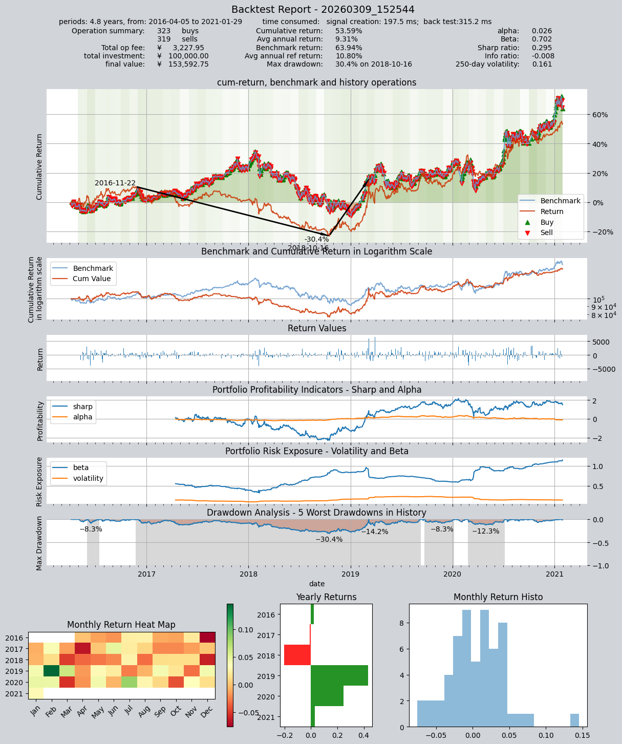
Results are as follows:
====================================
|                                  |
|         BACKTEST REPORT          |
|                                  |
====================================
qteasy running mode: 1 - History back testing
time consumption for operate signal creation: 197.5 ms
time consumption for operation back testing:  315.2 ms
investment starts on      2016-04-05 15:00:00
ends on                   2021-01-29 15:00:00
Total looped periods:     4.8 years.
-------------operation summary:------------
Only non-empty shares are displayed, call
"loop_result["oper_count"]" for complete operation summary
          Sell Cnt Buy Cnt Total Long pct Short pct Empty pct
000413.SZ    3        3       6    5.4%     -0.0%     94.6%
000415.SZ    1        1       2    2.0%     -0.0%     98.0%
000625.SZ    1        1       2    2.0%     -0.0%     98.0%
000629.SZ    1        1       2    1.5%     -0.0%     98.5%
000656.SZ    1        1       2    1.8%     -0.0%     98.2%
000723.SZ    5        5      10    8.2%     -0.0%     91.8%
000725.SZ    1        1       2    1.9%     -0.0%     98.1%
000728.SZ    1        1       2    1.9%     -0.0%     98.1%
000783.SZ    1        1       2    1.8%     -0.0%     98.2%
000898.SZ    4        4       8    7.1%     -0.0%     92.9%
...            ...     ...   ...      ...       ...       ...
001965.SZ    1        1       2    1.9%     -0.0%     98.1%
300418.SZ    2        2       4    3.8%     -0.0%     96.2%
300442.SZ    1        1       2    1.8%     -0.0%     98.2%
600026.SH    1        1       2    1.8%     -0.0%     98.2%
000975.SZ    1        1       2    1.8%     -0.0%     98.2%
300394.SZ    1        1       2    1.5%     -0.0%     98.5%
600160.SH    3        3       6    5.0%     -0.0%     95.0%
601127.SH    1        2       3    1.7%     -0.0%     98.3%
601058.SH    2        2       4    3.6%     -0.0%     96.4%
302132.SZ    1        1       2    2.0%     -0.0%     98.0%

Total operation fee:     ¥    3,227.95
total investment amount: ¥  100,000.00
final value:              ¥  153,592.75
Total return:                    53.59%
Avg Yearly return:                9.31%
Skewness:                          0.09
Kurtosis:                          6.81
Benchmark return:                63.94%
Benchmark Yearly return:         10.80%

------strategy loop_results indicators------
alpha:                            0.026
Beta:                             0.702
Sharp ratio:                      0.295
Info ratio:                      -0.008
250 day volatility:               0.161
Max drawdown:                    30.41%
    peak / valley:        2016-11-22 / 2018-10-16
    recovered on:         2019-03-07

trade log is stored in: /Users/jackie/Projects/qteasy_logs/trade_log_none_20260309_152544.csv
trade summary is stored in: /Users/jackie/Projects/qteasy_logs/trade_summary_none_20260309_152544.csv
value curve (complete values) is stored in: /Users/jackie/Projects/qteasy_logs/value_curve_none_20260309_152544.csv

==================END OF REPORT===================
11.4. Recap
In this tutorial, we explained in detail how to create your own trading strategy based on the trading strategy base class of qteasy through a specific example. Through this example, you can see that the trading strategy base class of qteasy provides sufficient flexibility to implement any type of trading strategy you can imagine.
Starting from the next tutorial, we will introduce the trading strategy optimization method of qteasy, find the optimal trading strategy parameters through various optimization algorithms, and evaluate the performance of the trading strategy.