9. Custom Strategies in qteasy

qteasy is a fully localized deployment and operation of quantitative trading analysis toolkits, with the following functions:

• Acquisition, cleaning, storage, processing, visualization, and use of financial data

• Create quantitative trading strategies and provide a large number of built-in basic trading strategies

• Vectorized high-speed trading strategy backtesting and trading result evaluation

• Optimization and evaluation of trading strategy parameters

• Deployment and live operation of trading strategies

You will learn the main functions and usage of qteasy through a series of practical examples in this series of tutorials.

9.1. Before you start

Make sure you have mastered the following before starting this tutorial:

• Install and configure qteasy —— QTEASY Tutorial 1

• Set up a local data source and have downloaded enough historical data to your local machine —— QTEASY Tutorial 2

• Learn to create trader objects and use built-in trading strategies —— QTEASY Tutorial 3

• Learn to use mixers to mix multiple simple strategies into more complex trading strategies —— QTEASY Tutorial 4

In the QTEASY documentation, you can find more information about using built-in trading strategies, creating custom strategies, and more. If you are not familiar with the basic usage of qteasy, you can go there to see more detailed instructions.

9.2. Target of this chapter

qteasy’s kernel is designed as a framework that balances high-speed

Meanwhile, qteasy’s backtesting framework has also been specially designed to completely avoid inadvertently importing “future functions” into your trading strategy, ensuring that your trading strategy is completely based on past data during backtesting, and also uses a lot of preprocessing techniques and JIT technology to compile key functions of the kernel to achieve a running speed comparable to that of C.

However, in order to achieve theoretically infinite possibilities of trading strategies, it may not be enough to use only built-in trading strategies and strategy mixing. Some specific trading strategies, or some particularly complex trading strategies cannot be created by mixing built-in strategies. This requires us to use the Strategy base class provided by qteasy to create a custom trading strategy based on certain rules.

In this chapter, we will introduce the trading strategy base class of qteasy, and explain in detail how to create a trading strategy that belongs only to you based on these base classes through several specific examples. To be progressive, we start with a relatively simple example.

9.3. Build a custom strategy

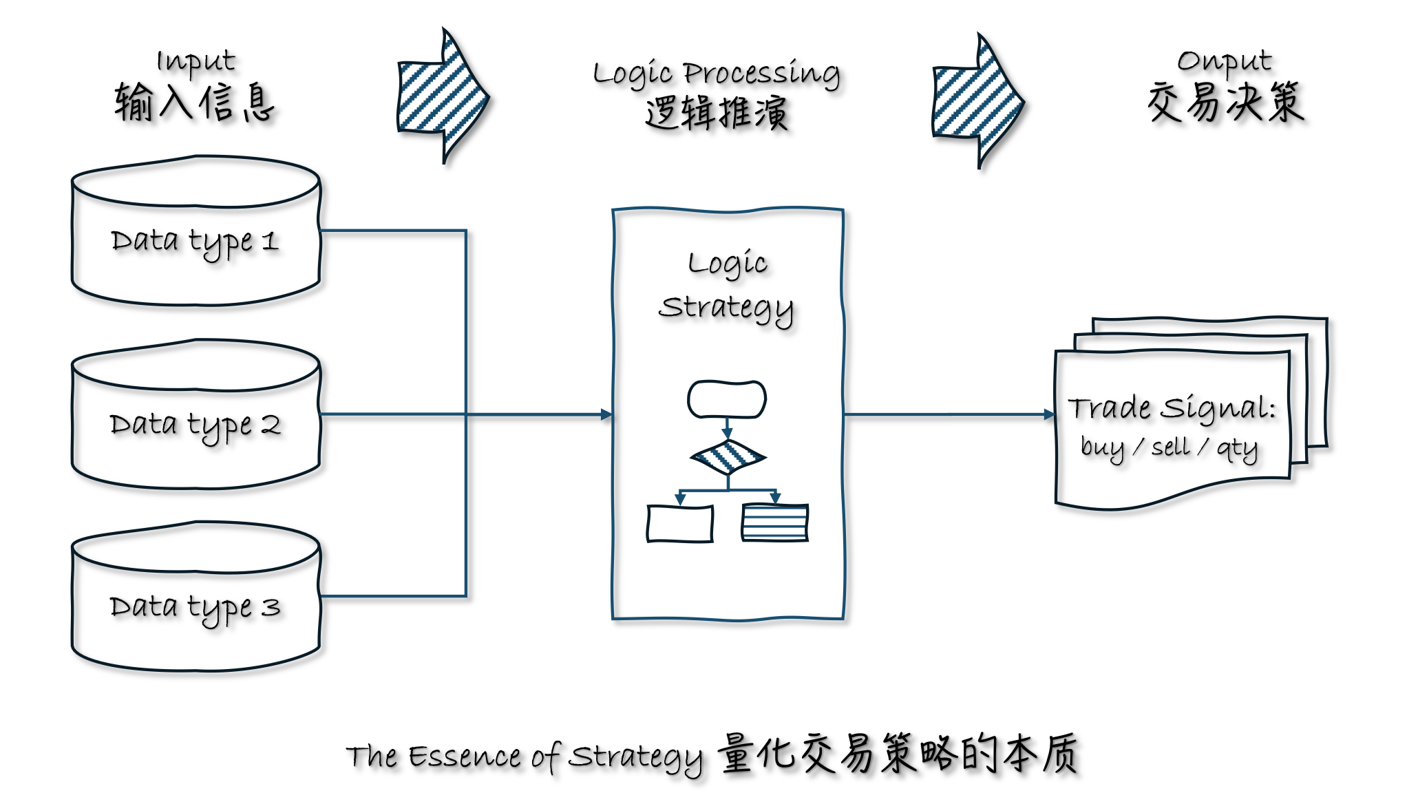
In the workflow of quantitative trading, a trading strategy is actually a function that takes known information as input and outputs trading decisions through a series of logical deductions. Regardless of the technical school, trading style, or analysis method, the most fundamental definition of a trading strategy is this.

For example:

• Technical analysts use past stock prices (input data) to calculate technical indicators (logical deduction) and make buy/sell decisions (trading decisions)

• Value investors use various indicators of listed companies (input data) to analyze the growth potential of the company (logical deduction) and decide which stock to buy/sell (trading decisions)

• Macro analysts, even if they don’t care about stock prices, need to refer to hot news, market sentiment (input data), analyze the overall market trend (logical deduction), and decide whether to enter the market (trading decisions)

• High-frequency or ultra-high-frequency arbitrage trading also needs to analyze the real-time changes in prices in the short term (input data), analyze the size of the arbitrage space (logical deduction), and intervene quickly in operations (trading decisions)

If a trading strategy tracks a small number of investment products at a high frequency, it is called a “timing trading strategy”; if it tracks a large number of investment products at a low frequency, it is called a “stock selection strategy”.

In short, all quantitative trading is a set of regularly run logical deductions, extracting the latest data as input each time it runs, and outputting a set of trading decisions. Repeatedly running in this way forms a stable trading operation flow, which is nothing more than the abstract concept of a trading strategy.

9.4. Use the Strategy strategy class in qteasy

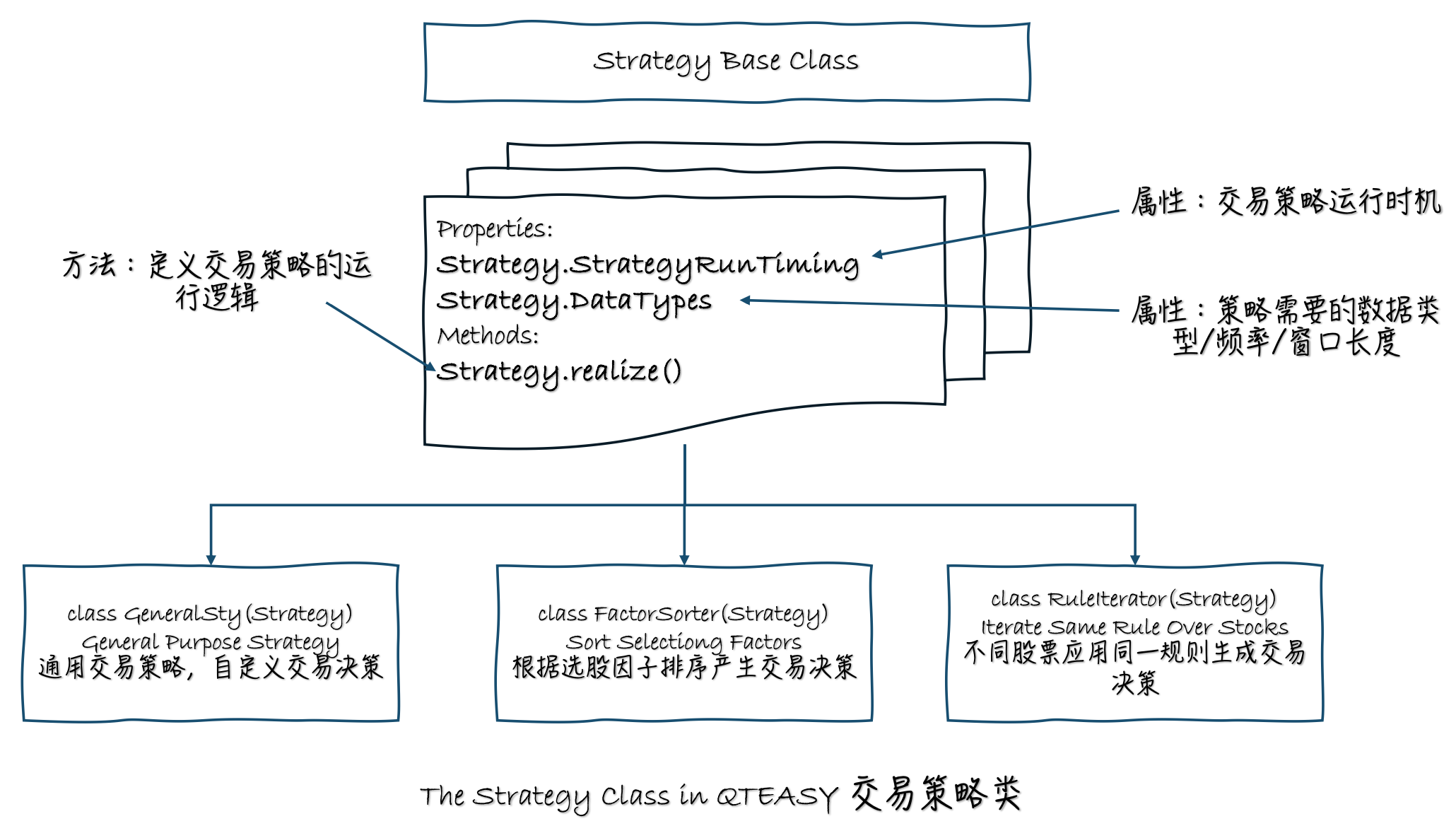
qteasy trading strategies are defined based on the concepts above. The strategy classes defined by qteasy are carriers of data and trading logic. By inheriting the Strategy class and defining your own strategy class—specifying the data the strategy needs and the strategy’s implementation logic within this class—you can create a custom trading strategy.

Therefore, in the design of qteasy, a trading strategy includes the following four core elements:

Strategies and strategy groups’ runtime timing

• Strategy runtime timing —— When a strategy runs and at what frequency it runs are determined by the strategy group. When adding a strategy to an Operator, you can specify the parameters run_freq and run_timing; together, these two parameters determine the strategy’s runtime timing.

A strategy’s tunable parameters and historical data

Trading strategies in qteasy also have a special design: tunable parameters. Tunable parameters are parameters that are continuously adjusted during strategy execution, such as the moving-average period, the number of stocks in a stock-picking ranking, and so on. These parameters directly affect the strategy’s performance, so we want to adjust them to find the optimal parameter combination, thereby achieving the best performance. qteasy provides a very convenient interface for defining tunable parameters. Users can define any number of tunable parameters in the strategy’s attributes, and specify a name, value range, data type, and so on for each tunable parameter. These defined tunable parameters will be automatically passed into the strategy implementation function, and users can directly use these parameters to implement trading logic.

• Tunable parameters of a strategy — parameters that need to be adjusted in a strategy, such as the moving-average period, the number of stocks in a stock-picking ranking, and so on. These parameters directly affect the strategy’s performance, so we want to adjust them to find the optimal parameter combination, thereby achieving the best performance. qteasy provides a very convenient interface, Parameters, for defining tunable parameters. Users can define any number of tunable parameters in the strategy’s attributes, and specify a name, value range, data type, and so on for each tunable parameter. These defined tunable parameters will be automatically passed into the strategy implementation function, and users can directly use these parameters to implement trading logic.

The data required by a strategy and its execution logic

• Data required by the strategy — the data inputs required by the strategy; for example, do you need daily candlestick (K-line) data for the past 10 days, or the P/E ratio for the past year? The amount of data required by the strategy can be defined completely freely via the Strategy.data_types attribute. Users can use the qt.StgData() object to define any type of data input. The data frequency and the window length can both be defined completely freely via strategy attributes, and qteasy will automatically package the data according to these definitions and feed it into the strategy’s implementation function.

• Strategy execution logic —— The strategy’s implementation logic is realized by overriding the Strategy.realize() method. Users can freely define how to use input data to generate trading signals.

A strategy’s output signals

qteasy allows users to define different types of trading signals: PT PS VS, etc. Users can choose different types of trading signals according to their needs to implement different types of trading strategies. The meanings of trading signals are briefly described below. To view a detailed introduction to different types of trading signals, see Trading Signals.

• PT-type signal —— Represents the percentage of position. The output is a value between 0 and 1, indicating what proportion of the position to hold. For example, an output of 0.5 means holding 50% of the position; 0 means holding none; 1 means fully invested;

• PS signal — represents the trading percentage. The output is a value between -1 and 1, indicating what proportion of the position to buy/sell. For example, an output of 0.5 means buy 50% of the position, -0.5 means sell 50% of the position, and 0 means no action;

• VS-type signal —— Represents the trade quantity. The output number indicates the number of shares to buy/sell; for example, 500 means buying 500 shares, and -300 means selling 300 shares.

Except for the information related to the strategy above, all other work has been done by qteasy, and all trading data will be automatically packaged into an ndarray array according to the strategy attributes, which can be easily extracted and used; the same trading strategy will automatically extract trading data during live operation, generate trading signals according to the defined strategy, and automatically extract historical data during backtesting, generate historical data slices, and will not form future functions. At the same time, all trading data will

Therefore, customizing strategies in qteasy is very simple:

• __init__() Define all parameters of the strategy in this method, including the strategy’s name, description, and, most importantly, tunable parameters, data types, etc. These parameters will be automatically recognized by qteasy and can be used directly when the strategy runs.

• realize() Define the strategy’s execution logic in this method: extract historical data and generate trading signals based on the data.

In addition to the strategy attributes mentioned above, a custom strategy also has the same basic attributes as built-in trading strategies, such as tunable parameters, etc. Since they are the same as those of built-in trading strategies, they will not be repeated here.

9.5. There are three different custom strategy base classes

Three different strategy classes are provided by qteasy to facilitate users to create custom strategies for different situations.

• GeneralStg: General trading strategy class, users need to provide trading decision signals for all trading assets in the realize() method

• FactorSorter: Factor stock selection class, users only need to define the stock selection factor in the realize() method, and multiple stock selection actions can be implemented through object attributes

• RuleIterator: Rule Iterator class, users only need to define stock selection or timing rules for a stock, and the same rules will be cyclically applied to all stocks, and different stocks can define different parameters

Three trading strategy base classes have exactly the same attributes and methods, the only difference is in the definition of the realize() method.

Now, Let’s learn how to create custom strategies through a few progressive examples.

9.6. Define a dual moving average timing trading strategy

Our first example is the simplest dual moving average timing trading strategy, which is the most classic timing trading strategy. This moving average timing strategy has two adjustable parameters:

• FMA Fast moving average period

• SMA Slow moving average period The strategy calculates the simple moving average generated by the above two periods based on the closing price of the past period. When the two moving averages cross, a trading signal is generated:

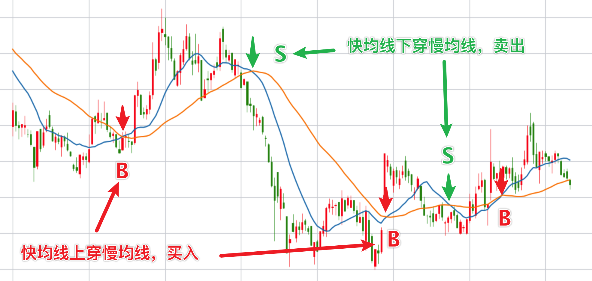
• When the fast moving average crosses the upper boundary from bottom to top, a full buy signal is issued

• When the fast moving average crosses the upper boundary from top to bottom, a full sell signal is issued

The logic of this strategy is very simple. So how do we define this strategy? First, we need to decide which type of trading strategy base class to use. In many cases, all three trading strategy base classes can be used to generate the same trading strategy, but some base classes have made some definitions in advance for specific types of strategies, which can further simplify the code of the strategy. This strategy is a typical timing strategy, which is a strategy type that applies the same rule to different investment products, so we can use the RuleIterator strategy class to establish the strategy. In the following examples, we will talk about the other two strategy classes.

Now, let’s clarify the three main elements of this strategy:

• Timing of the strategy —— For simplicity, we define that this strategy runs at the close of each day

• Data required by the strategy ——To calculate the two moving averages, we need the historical closing price (“close”) each time the strategy runs, and we need at least SMA days of historical data to calculate the SMA slow moving average

• Logic of the strategy ——After extracting the closing price, first calculate the two moving averages, and then determine whether the moving average of the most recent day has crossed up/down. Specifically, it is to compare the relative relationship between the two moving average prices of yesterday and today. If the SMA was greater than the FMA yesterday, and today the SMA is less than the FMA, it means that the FMA has crossed the SMA from below, and a full buy signal should be generated. This signal is 1. If the situation is exactly the opposite, a full sell signal of -1 is output. In other cases, 0 is output, and there is no trading signal.

With the above preparation, let’s see how the strategy code is defined. The first step in a basic strategy code is to inherit the strategy base class (here it is RuleIterator) and create a custom class:

from qteasy import RuleIterator
from qteasy import Parameter, StgData

class Cross_SMA(RuleIterator):

    # 策略的属性定义在__init__()方法中
    def __init__(self):
        super().__init__(
        )

    # 策略的具体实现代码写在策略的realize()函数中
    def realize(self):
        """策略的具体实现代码：
        """
        pass

OK, the above few lines of code are the entire framework of our first custom trading strategy. Fill in the attributes and supplement the logic in this framework to become a complete trading strategy. How to do it? First, define the most basic attributes of this strategy — name, description, and adjustable parameters:

Name and description are both information about the strategy, which is convenient for understanding the purpose of the strategy when called later. We can define them according to our preferences. The more critical attribute is the adjustable parameters.

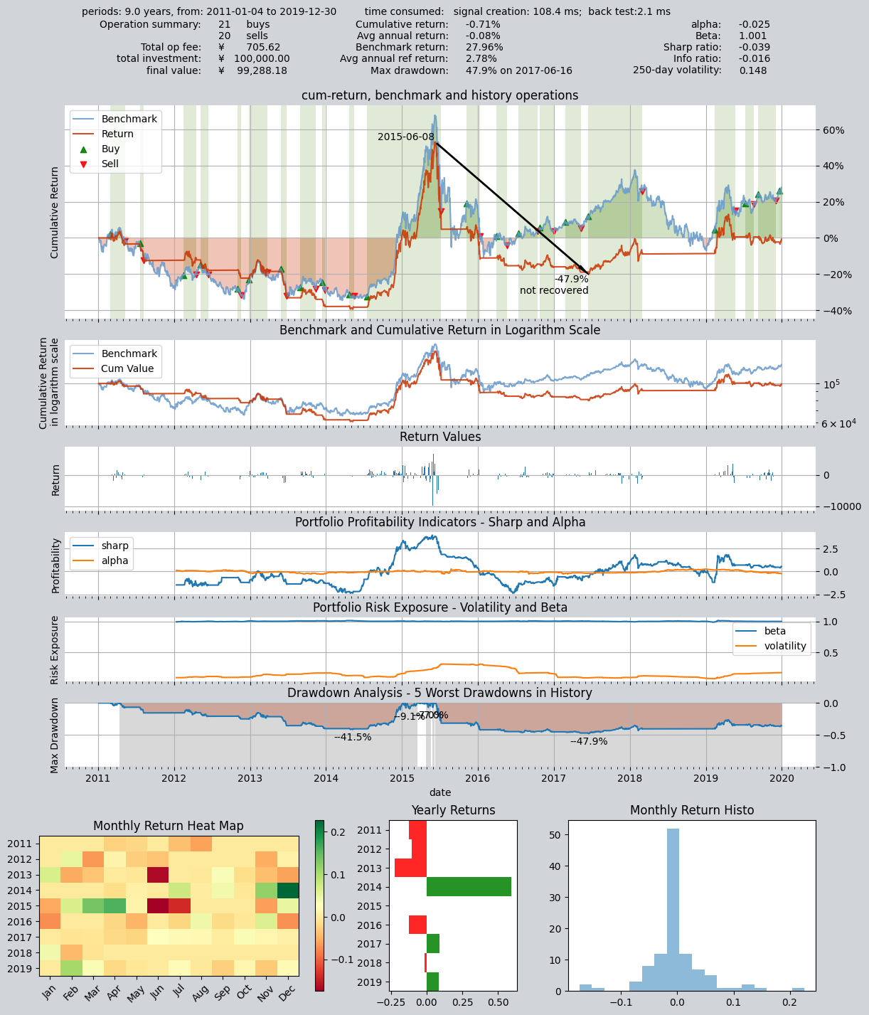
In this custom strategy, we want the calculation parameters of the fast moving average and the slow moving average to be adjustable, because these two parameters directly affect the specific positions of the fast and slow moving averages, which directly affect the intersection points of the two moving averages, thus forming different buying and selling points. See the following two figures, which show the intersection of different speed moving averages of the same stock at the same time. When the calculation period of the moving average is different, the buying and selling points generated are completely different:

The moving average periods in the above figure are 15 days/40 days, generating three buy signals and two sell signals 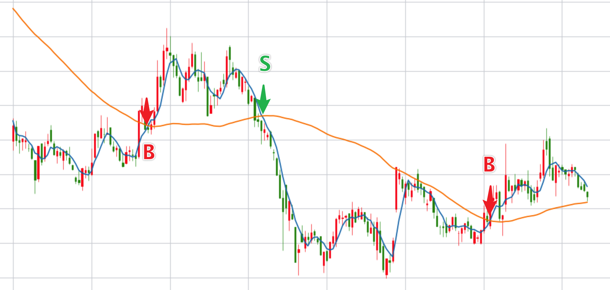The moving average periods in the above figure are 5 days/50 days, generating two buy signals and one sell signal

Since the moving average period directly affects the performance of the strategy, we naturally hope to find the best combination of moving average periods (parameter combinations) to make the strategy perform best. To achieve this goal, qteasy allows users to define these parameters as “adjustable parameters” and provides optimization algorithms to find the best parameters. For all built-in trading strategies, the number and meaning of adjustable parameters are defined and cannot be modified by users. However, in custom strategies, users have a lot of freedom. In theory, any variable used in the strategy running process can be defined as an adjustable parameter.

Here, we define the periods of the fast and slow moving averages as adjustable parameters, and define them in the strategy attributes as follows

A strategy’s tunable parameters are defined using Parameter objects. With these objects, we can specify a name, value range, data type, and so on for each tunable parameter. These defined tunable parameters will be automatically passed into the strategy implementation function, and users can directly use them to implement trading logic.

pars=[Parameter((10, 100), data_type='int', name='fast', value=30),
      Parameter((10, 100), data_type='int', name='slow', value=60)],  # 策略默认参数是快均线周期30， 慢均线周期60

Define the data required by the strategy

The data required by the strategy is determined by the StgData object. In qteasy, each data-type object can be identified by a unique ID, data frequency, and asset type. You can also specify the length of the data window.

With data defined, qteasy will automatically package the data within the window and send it to the strategy realize() function. If all historical data is packaged into a series of data windows according to the same rules during backtesting, the historical data format received by the realize() function is completely the same, and the processing method is completely the same, ensuring the consistency of live and backtesting operations, and also avoiding the future functions that may occur during backtesting:

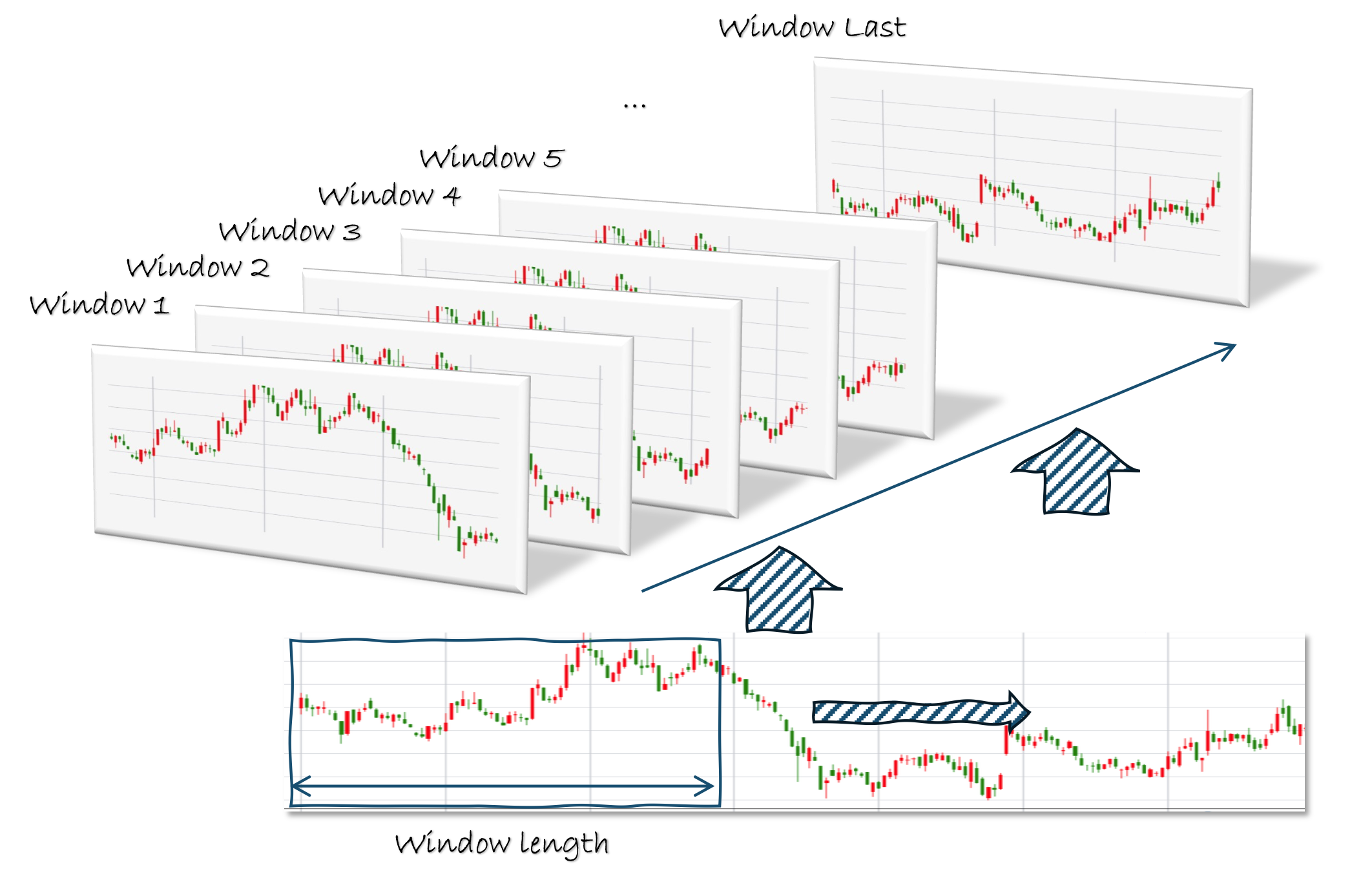
The definition of the StgData data type is as follows. We need the daily closing prices for the past 201 days. The reason we need 201 days of closing prices is that we defined the maximum range of the tunable parameter as 200; to calculate a moving average with a period of 200, we need 201 days of closing prices.

data_types=[StgType('close', asset_type='ANY', freq='d', window_length=201)]  # 策略基于收盘价计算均线，因此数据类型为'close'，历史数据的频率为日，历史数据窗口长度为201，每一次交易信号都是由它之前前201天的历史数据决定的

Based on the data types defined above, qteasy assigns this strategy a unique ID: close_ANY_d. With this ID, you can retrieve historical data in the strategy implementation function; we will introduce how to retrieve historical data later.

Now, all the important attributes of the custom trading strategy have been defined. Next, we will define the implementation of the strategy.

Realization of custom trading strategy: realize()

In the realize() method, we need to do three things, and we solve them one by one:

• Acquire historical data

• Acquire adjustable parameters

• Create algorithm and define output

Acquire historical data and adjustable parameter values:

As mentioned earlier, this strategy’s tunable parameter is the moving-average lookback period. Therefore, to use the tunable parameter as the calculation period, we need to obtain the tunable parameter’s value as well as the specific historical data.

In the realize() method, it is very easy to obtain tunable parameters and historical data: use self.get_data() and self.get_pars() respectively. Both methods can retrieve multiple data series or parameters at once; the retrieved values will be unpacked into a tuple, which users can use directly.

def realize(self):
    """策略的具体实现代码
    """
    close = self.get_data('close_ANY_d')  # 通过数据ID获取数据：最近201天的收盘价
    f, s = self.get_pars('fast', 'slow')  # 读取快均线（fast）和慢均线（slow）的计算周期

Now, all the elements needed to implement the strategy logic are ready, and we can start implementing the strategy logic.

We first need to calculate two sets of moving averages. If the user has installed the ta-lib library, we can directly call ta-lib’s SMA function to calculate moving averages. If it is not installed, that is not a big problem, because qteasy provides a ta-lib-free version of the SMA function (not all technical indicators have a ta-lib-free version; see the reference documentation for details), which can be imported and used directly.

def realize(self, h, **kwargs):
    """策略的具体实现代码
    """
    ...
    from qteasy.tafuncs import sma
    # 使用qt.sma计算简单移动平均价
    s_ma = sma(close, s)
    f_ma = sma(close, f)
    # 为了考察两条均线的交叉, 计算两根均线昨日和今日的值，以便判断
    s_today, s_last = s_ma[-1], s_ma[-2]
    f_today, f_last = f_ma[-1], f_ma[-2]

Calculate the moving average, we can directly define the output of the strategy in the realize method, that is, the trading decision.

For the RuleIterator class strategy, no matter how many stocks our strategy acts on at the same time, we only need to define one set of rules, which is called “rule iteration”, so we only need to output a number to represent the trading decision. This number will be automatically converted into different trading orders by qteasy. The conversion rules are determined by the working mode of the Operator object, which has been introduced in the previous tutorials and will not be repeated here.

In this example, we plan to have the signals output by the trading strategy represent what proportion of total assets to invest in the investment instrument. Then we only need to generate a trading signal “1” on the day we should buy, generate a trading signal “-1” on the day we should sell, and output “0” if we do not want to trade:

def realize(self, h, **kwargs):
    """策略的具体实现代码
    """
    ...
    if (f_last < s_last) and (f_today > s_today):  
        # 当快均线自下而上穿过上边界（即昨日快均线低于慢均线，而今天高于于慢均线），发出全仓买入信号
        return 1
    elif (f_last > s_last) and (f_today < s_today): 
        # 当快均线自上而下穿过上边界（即昨日快均线高于慢均线，而今天低于于慢均线），发出全部卖出信号
        return -1
    else:  # 其余情况不产生任何信号
        return 0

Now, we have finished the definition of a strategy! qteasy will complete all the complex work behind the scenes, and users only need to focus on solving the data and logic definitions of the strategy. The complete code is as follows (to save space, all comments are deleted):

from qteasy import RuleIterator, Parameter, StgData
from qteasy.tafuncs import sma
# 创建双均线交易策略类
class Cross_SMA_PS(RuleIterator):
    def __init__(self):
        super().__init__(
            name='CROSSLINE',  # 策略的名称
            description='快慢双均线择时策略',  # 策略的描述
            pars=[Parameter((10, 100), par_type='int', name='fast', value=30),
                  Parameter((10, 100), par_type='int', name='slow', value=60)],
            data_types=[StgData('close', freq='d', asset_type='ANY', window_length=201)],
        )

    def realize(self):
        
        close = self.get_data('close_ANY_d')  # 通过数据ID获取数据：最近201天的收盘价
        f, s = self.get_pars('fast', 'slow')  # 读取快均线（fast）和慢均线（slow）的计算周期
        
        # 使用qt.sma计算简单移动平均价
        s_ma = sma(close, s)
        f_ma = sma(close, f)
        # 为了考察两条均线的交叉, 计算两根均线昨日和今日的值，以便判断
        s_today, s_last = s_ma[-1], s_ma[-2]
        f_today, f_last = f_ma[-1], f_ma[-2]
        
        if (f_last < s_last) and (f_today > s_today):  
            # 当快均线自下而上穿过上边界（即昨日快均线低于慢均线，而今天高于于慢均线），发出全仓买入信号
            return 1
        elif (f_last > s_last) and (f_today < s_today): 
            # 当快均线自上而下穿过上边界（即昨日快均线高于慢均线，而今天低于于慢均线），发出全部卖出信号
            return -1
        else:  # 其余情况不产生任何信号
            return 0

Next, we can use this custom strategy just like any built-in trading strategy.

We need to create a new Operator object, and when creating it, add the Cross_SMA strategy we just created into the Operator, while specifying this strategy’s signal type as PS. This tells the Operator to use the PS rules to interpret the signals generated by the trading strategy:

op = qt.Operator(strategies=[Cross_SMA_PS()], signal_type='PS')

Let’s take a look at the backtest results of this strategy.

Backtest results of the first strategy

The parameter settings for backtesting the strategy are exactly the same as for built-in trading strategies

op = qt.Operator([Cross_SMA_PS()], signal_type='PS')

# 设置op的策略参数
op.set_parameter(0, 
                 par_values= (20, 60)  # 设置快慢均线周期分别为20天、60天
                )

# 设置基本回测参数，开始运行模拟交易回测
res = qt.run(op, 
             mode=1,  # 运行模式为回测模式
             asset_pool='000300.SH',  # 投资标的为000300.SH即沪深300指数
             invest_start='20110101',  # 回测开始日期
             invest_end='20191231', # 回测结束日期
             visual=True  # 生成交易回测结果分析图
            )

Results of backtesting are as follows:

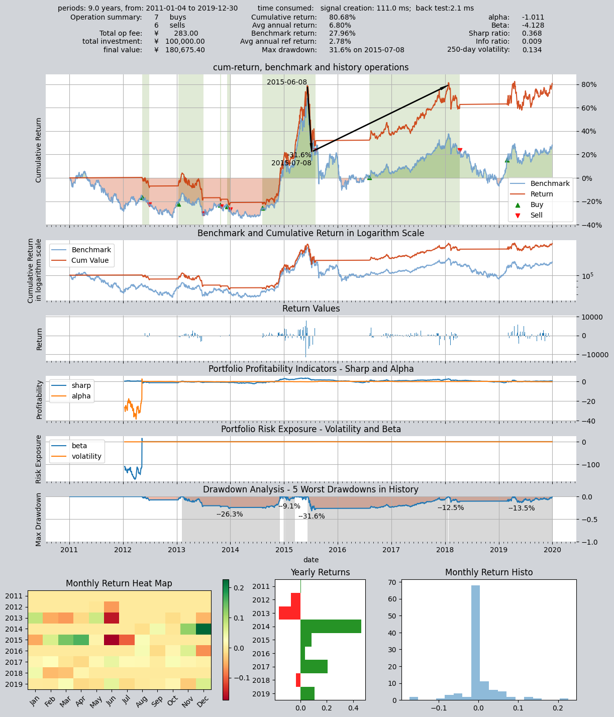
Now, we can try to modify the adjustable parameters of the strategy and run the backtest again. The backtest interval is the same as the previous one:

op.set_parameter(0, 
                 par_values= (25, 166)  # 设置快慢均线周期分别为25天、166天
                )

# 设置基本回测参数，开始运行模拟交易回测，回测参数完全一样
res = qt.run(op, 
             mode=1,  # 运行模式为回测模式
             asset_pool='000300.SH',  # 投资标的为000300.SH即沪深300指数
             invest_start='20110101',  # 回测开始日期
             visual=True  # 生成交易回测结果分析图
            )

As you can see, the backtest results of the strategy have changed significantly after changing the parameters: To learn how to optimize strategy parameters, please refer to the following chapters of this tutorial

====================================
|                                  |
|         BACKTEST REPORT          |
|                                  |
====================================
qteasy running mode: 1 - History back testing
time consumption for operate signal creation: 111.0 ms
time consumption for operation back testing:  2.1 ms
investment starts on      2011-01-04 15:00:00
ends on                   2019-12-30 15:00:00
Total looped periods:     9.0 years.
-------------operation summary:------------
Only non-empty shares are displayed, call 
"loop_result["oper_count"]" for complete operation summary
          Sell Cnt Buy Cnt Total Long pct Short pct Empty pct
000300.SH    6        7      13   46.8%     -0.0%     53.2%  

Total operation fee:     ¥      283.00
total investment amount: ¥  100,000.00
final value:              ¥  180,675.40
Total return:                    80.68% 
Avg Yearly return:                6.80%
Skewness:                         -1.01
Kurtosis:                         17.32
Benchmark return:                27.96% 
Benchmark Yearly return:          2.78%

------strategy loop_results indicators------ 
alpha:                           -1.011
Beta:                            -4.128
Sharp ratio:                      0.368
Info ratio:                       0.009
250 day volatility:               0.134
Max drawdown:                    31.58% 
    peak / valley:        2015-06-08 / 2015-07-08
    recovered on:         2018-01-22

==================END OF REPORT===================

At this point, we have implemented a simple custom timing trading strategy. So how do we implement the other two strategy classes? We will use more examples to explain in the next chapter.

9.7. Recap

In this section, we learned about the abstract definition of trading strategies in qteasy, understood the basic elements contained in a trading strategy and their definition methods, and created a custom dual moving average trading strategy through the simplest example.

As next step, we will continue to introduce custom trading strategies. Because there is a lot of related content, the tutorials related to custom trading strategies will occupy three chapters. In the next chapter, we will learn how to use the other two custom strategy base classes (FactorSorter factor stock selection base class and GeneralStg general strategy base class) to create trading strategies. Then, we will use another chapter to introduce a more complex custom trading strategy to show the flexibility of qteasy. See you in the next section!