QTEASY Quick Start Guide
Install and import
使用 pip 安装(要求 Python >= 3.9, <3.13):部分功能(如全部内置策略、数据库存储等)需要可选依赖,详见 FAQ 与安装说明。
pip install qteasy
After startup, you can import qteasy and check the version number:
>>> import qteasy as qt
>>> print(qt.__version__)
The output is as follows:
2.6.0
qteasy release history — Change notes for each version, which can be viewed before upgrading.
Get it running in one minute
In this section, you will complete: configure the tushare Token → download ten years of CSI 300 index data → view the data and candlestick chart → run a timing backtest on 000300.SH using the built-in DMA strategy, and obtain a usable backtest result.
2. 下载 000300.SH 十年指数数据
After configuring the tushare Token, download the daily data of the CSI 300 Index (000300.SH). It is recommended to download the trading calendar and the index basic information first, and then download the index daily data (about ten years):
Using the qteasy.refill_data_source() function, qteasy will automatically download data from the configured data source. When the data volume is too large, it will automatically download in chunks, perform data checks and cleaning, and store it in the database.
>>> # 下载交易日历与指数基础信息
>>> qt.refill_data_source(tables=['trade_calendar', 'index_basics'])
>>> # 下载 000300.SH 近十年日线数据
>>> qt.refill_data_source(
...     tables=['index_daily'],
...     start_date='20140101',
...     end_date='20241231',
...     symbols=['000300.SH'],
... )
The output is as follows:
Filling data source file://csv@qt_root/data/ ...
into 1 table(s) (parallely): {'trade_calendar'}
<trade_calendar> 35000 wrn: 100%|█████████████████████████████████████████████████████| 8/8 [00:05<00:00,  1.58task/s]
Data refill completed! 35000 rows written into 1/1 table(s)!

Filling data source file://csv@qt_root/data/ ...
into 2 table(s) (parallely): {'index_daily', 'index_basic'}
<index_daily> 152760 wrn: 100%|███████████████████████████████████████████████████████| 2/2 [00:05<00:00,  2.51s/task]
<index_basic> 1327 wrn: 100%|█████████████████████████████████████████████████████████| 8/8 [00:05<00:00,  1.58task/s]
Data refill completed! 154087 rows written into 2/2 table(s)!
3. 查看数据与 K 线图
After the data has been stored locally, you can fetch it with get_history_data, plot candlesticks with HistoryPanel.plot and qt.candle, and verify whether the data and quotes are normal:
>>> # 获取近一年日线,直接返回 HistoryPanel
>>> hp = qt.get_history_data(
... htypes='open, high, low, close', # 需要获取的数据类型分别为开盘价、最高价、最低价、收盘价
... shares='000300.SH', # 资产类型为沪深300指数
... start='20230101', # 数据起始日期
... end='20231231', # 数据结束日期
... )
>>> print(hp) # 查看数据结构与范围
>>> # 在 HistoryPanel 上绘制静态 K 线 + 成交量
>>> hp.plot(interactive=False)
>>> # 或者使用 qt.candle 快速绘制 K 线(内部同样基于 HistoryPanel)
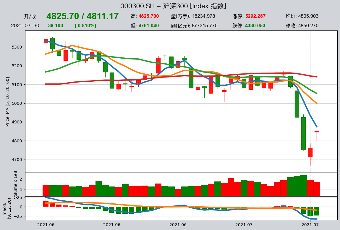
>>> qt.candle('000300.SH', start='2023-06-01', end='2023-12-01', asset_type='IDX')
3.1 Interactive charts (Plotly) and dependencies
If you want to zoom, pan, and view the specific values corresponding to each candlestick/indicator in a Notebook, you can use interactive plotting:
>>> hp.plot(interactive=True)
Interactive charts rely on Plotly. It is recommended to choose the installation based on your usage environment:
Basic interaction (Plotly Figure):
pip install plotly
More complete interaction in Notebook (FigureWidget + callbacks):
pip install ipywidgets anywidget
In a Notebook, qteasy will first try to provide a more complete FigureWidget experience; if the current kernel/dependencies do not meet the requirements, it will fall back to HTML display. If Plotly is not installed, interactive=True will directly raise an English error message (usually containing “requires plotly”).
3.2 Most commonly used interactive parameters
plotly_backend_app='auto'|'FigureWidget'|'html': Select the output mode in a Notebook (default is'auto').layout='auto'|'overlay'|'stack': multi-asset layout.'overlay'is most commonly used for overlay comparisons of two assets only;'auto'will automatically choose between “two assets → overlay, otherwise → stack”.highlight='max'|'min': Highlight the maximum/minimum value point (available for both static and interactive plots).
The output is as follows:
{'000300.SH':
               open     high      low    close
2023-01-03  3864.84  3893.99  3831.25  3887.90
2023-01-04  3886.25  3905.90  3873.65  3892.95
2023-01-05  3913.49  3974.88  3912.26  3968.58
...             ...      ...      ...      ...
2023-10-10  3696.25  3701.26  3655.59  3657.13
2023-10-11  3674.75  3689.53  3658.35  3667.55
2023-10-12  3697.93  3711.50  3682.84  3702.38

[186 rows x 4 columns]
}
3.5 Working with historical data (HistoryPanel)
In practical research, many times we not only need to “look at candlestick charts,” but also need to compute statistics on historical data and generate factors in code. In addition to returning a DataFrame, get_history_data() can also directly return a 3D HistoryPanel, making it easy to perform unified calculations across multiple instruments and multiple indicators:
>>> # 获取 000300.SH 的 OHLCV 历史数据,并返回 HistoryPanel
>>> hp = qt.get_history_data(
...     htypes='open, high, low, close, vol',
...     shares='000300.SH',
...     start='20230101',
...     end='20231231',
...     as_data_frame=False,          # 关键:返回 HistoryPanel
... )
>>> print(hp.shape, hp.shares, hp.htypes)

>>> # 1) 计算简单收益率矩阵(时间 × 股票)
>>> ret = hp.returns(price_htype='close', method='simple')
>>> print(ret.head())

>>> # 2) 计算 20 日滚动波动率
>>> vol = hp.volatility(window=20, price_htype='close', annualize=True)
>>> print(vol.tail())

>>> # 3) 生成 K 线技术指标(如 20 日均线、MACD)
>>> hp_ma = hp.kline.sma(window=20)              # 在 htypes 中新增 'sma_20'
>>> hp_ma_macd = hp_ma.kline.macd()              # 再追加 MACD 指标
>>> print(hp_ma_macd.htypes)

>>> # 4) 识别蜡烛形态(如锤头线)
>>> hammer = hp.candle_pattern('cdlhammer')      # 返回 DataFrame,非 0 代表出现形态
>>> print(hammer[hammer['000300.SH'] != 0].head())

>>> # 5) 单只股票切片成 DataFrame,方便与 pandas / sklearn 等联动
>>> df_300 = hp_ma_macd.to_share_frame('000300.SH')
>>> print(df_300.tail())
The example above demonstrates how, after obtaining a HistoryPanel from get_history_data(..., as_data_frame=False), you can compute returns, volatility, technical indicators, and pattern signals in just one or two lines of code, and switch back at any time to the familiar DataFrame for further analysis.
For a more systematic guide to using HistoryPanel, see the “Operations and Analysis of Historical Data” chapter in the “User Guide”, as well as the HistoryPanel API Reference.
4. 使用 DMA 策略做择时回测
Use the built-in DMA moving-average timing strategy, with 000300.SH as the trading instrument, and run a backtest on the downloaded 10 years of data. Below, we use a set of commonly used and relatively stable parameters (short MA 20, long MA 60, DMA period 10) to directly obtain the backtest results and charts:
>>> # 设置qteasy的运行配置参数
>>> qt.configure(
...     asset_pool='000300.SH',  # 交易资产池包括沪深300指数
...     asset_type='IDX',  # 投资资产类型为IDX-指数
...     invest_cash_amounts=[100000],  # 回测初始投资金额为十万元
...     invest_start='20150101',  # 回测投资初始日期
...     invest_end='20241231',  # 回测投资结束日期
...     cost_rate_buy=0.0003,  # 交易费率:买入手续费万分之三
...     cost_rate_sell=0.0001,  # 交易费率:卖出手续费万分之一
...     visual=True,  # 是否输出回测结果可视化图表:是
...     trade_log=True,  # 是否输出回测记录:是
... )
>>> op = qt.Operator(strategies='dma')  # 创建一个交易员对象,执行一个DMA交易策略
>>> op.set_parameter('dma', par_values=(20, 60, 10))  # 设置交易策略的参数
>>> res = qt.run(op, mode=1)  # 启动交易,运行模式为1(回测交易)
The output is as follows:
====================================
|                                  |
|         BACKTEST REPORT          |
|                                  |
====================================
qteasy running mode: 1 - History back testing
time consumption for operate signal creation: 81.3 ms
time consumption for operation back testing:  4.9 ms
investment starts on      2015-01-05 15:00:00
ends on                   2024-12-30 15:00:00
Total looped periods:     10.0 years.
-------------operation summary:------------
Only non-empty shares are displayed, call
"loop_result["oper_count"]" for complete operation summary
          Sell Cnt Buy Cnt Total Long pct Short pct Empty pct
000300.SH   340       41    381   44.7%     -0.0%     55.3%

Total operation fee:     ¥    3,261.19
total investment amount: ¥  100,000.00
final value:              ¥  115,601.73
Total return:                    15.60%
Avg Yearly return:                1.46%
Skewness:                         -1.16
Kurtosis:                         16.95
Benchmark return:                 1.67%
Benchmark Yearly return:          0.17%

------strategy loop_results indicators------
alpha:                            0.006
Beta:                             0.975
Sharp ratio:                      0.113
Info ratio:                       0.001
250 day volatility:               0.130
Max drawdown:                    36.85%
    peak / valley:        2015-04-27 / 2018-11-27
    recovered on:         Not recovered!


==================END OF REPORT===================
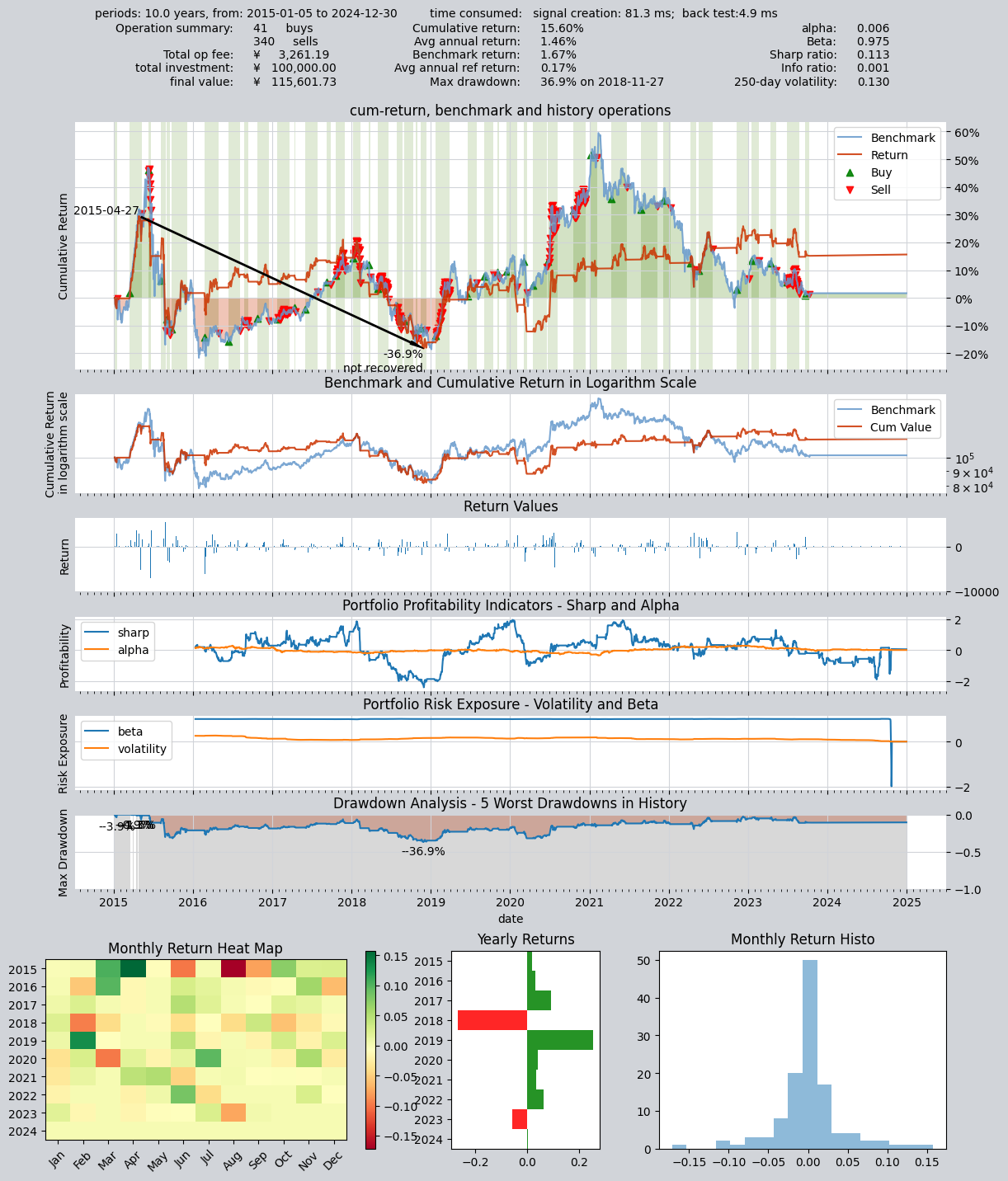
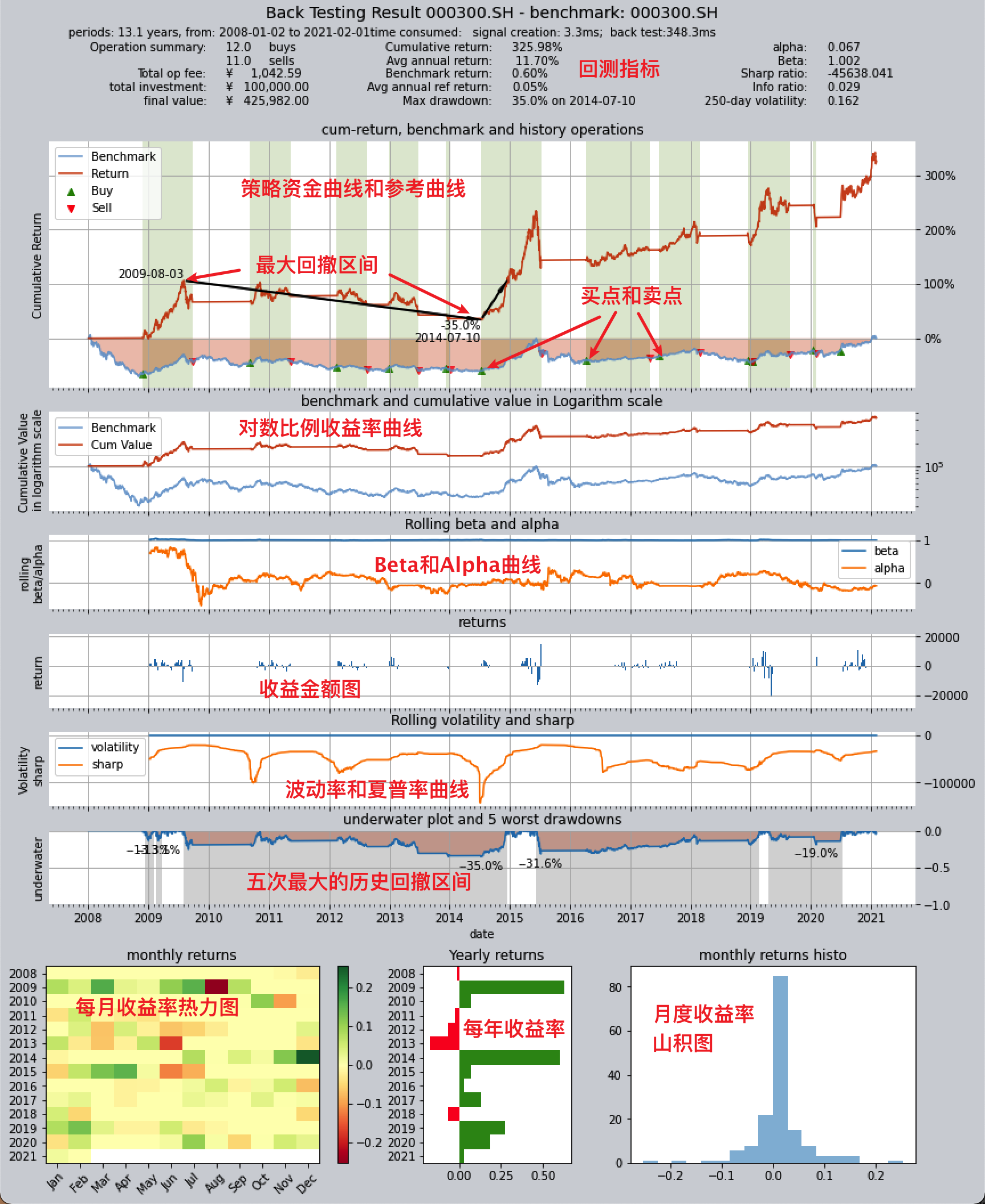
After running, you will get evaluation metrics such as the equity curve, maximum drawdown, and Sharpe ratio, along with visualized charts. To try other parameters or optimize ranges, refer to the next section “What can qteasy do” for parameter optimization and the backtesting documentation.
What can qteasy do?
Fetch and manage historical financial data:
Conveniently obtain large amounts of historical financial data from multiple sources, clean the data, and store it locally in a unified format
Use the
DataTypeobject to manage available information in financial data in a structured way. Even for complex information such as adjusted prices and index constituents, you can retrieve it with just one line of code.Financial data visualization, statistical analysis, and visualization of analysis results based on
DataTypeobjectsStore data locally and retrieve it on demand, providing a consistent data foundation for backtesting and live trading, making results easier to reproduce
Create trading strategies in a simple and safe way
With the
BaseStrategyclass, the method for defining trading strategies is intuitive and the logic is clear.Over 70 built-in strategies out of the box, plus a unique strategy mixing and grouping mechanism—complex strategies can be assembled from simple ones, like building with blocks.
The data inputs and usage methods of trading strategies are fully encapsulated and secure, completely avoiding issues such as inadvertently introducing future functions and data leakage, ensuring the authenticity and reliability of strategy results.
The same strategy logic is used for both backtesting and live trading, reducing the gap between “great backtest results” and “underwhelming live performance.”
Backtest evaluation, optimization, and simulated automated trading for trading strategies
Manage strategy execution through the
Operatortrader class, backtest strategies according to the real market trading rhythm, evaluate trading results comprehensively across multiple dimensions, and generate trading reports and result charts.Provides multiple optimization algorithms, including simulated annealing, genetic algorithms, Bayesian optimization, etc., to optimize strategy performance in large parameter spaces.
Fetch real-time market data, run strategy simulations for automated trading, and track and record information such as trading logs, stock positions, and account balance changes.
Backtesting, optimization, and live trading use the same execution mechanism: write a strategy once and run it in all modes, with clear configuration for easy reproduction and troubleshooting.
In the future, we will connect to brokers’ live trading interfaces via the QMT API to enable automated trading.
End-to-end roadmap / tutorial
If you want to follow the complete workflow from “configuration to backtesting, optimization, and simulation/live trading,” you can read the tutorials and documentation in the following order. Each step has corresponding sections and examples:
Configure data sources and Token → Tutorial: Getting Started, Tutorial: Getting Data
下载数据 → 教程:获取数据、下载并管理金融历史数据 2b. 玩数据与简单因子(可选,建议策略回测前完成) → 教程 2.0 最小数据集 → 教程 2.5 §0 三十分钟闭环 →(进阶)2.6 / 2.7 / 2.8;可运行
examples/data_playground_e2e.pyDefine a Strategy and Backtest → Tutorial: Your First Strategy, Tutorial: Built-in Strategies, Tutorial: Custom Strategies, How to Run a Backtest
Parameter Optimization → Tutorial: Optimizing Trading Strategies, Optimize Trading Strategies
Simulation/Live Trading → Tutorial: Deploying and Running Trading Strategies, Simulation/Live Trading Overview
The tutorials above already cover the complete chain from configuration to backtesting, optimization, and simulation/live trading; if you run into issues, you can check the FAQ for common explanations such as “how to get it running end-to-end,” “why it’s slow,” and “avoiding look-ahead bias.”
Next
Tutorial: Get Data — Configure data sources and download more data
教程:HistoryPanel 玩数据 — §0 三十分钟因子研究闭环
Tutorial: Your First Strategy — Use built-in strategies and run backtests
Backtesting and Evaluation — Backtest parameters and how to interpret results
API Reference — Complete interface documentation