3. Collective Bidding Strategy
Reference source: docs/_joinquant_migration_source/Example_03_集集竞价选股.ipynb The first Markdown cell.
This strategy obtains the constituent stock data of SHSE.000300 Shanghai and Shenzhen 300 and counts the number of days when the opening price is greater than the previous closing price within 30 days. When this number exceeds the threshold of 10, it is added to the stock pool. Then, close the positions of stocks not in the stock pool and equally allocate the stocks in the stock pool. The trading interval is one month.
Back test data: SHSE.000300 Shanghai and Shenzhen 300 Index component stocks Backtest time: 2016-04-05 to 2021-02-01
>>> import qteasy as qt
>>> import pandas as pd
>>> import numpy as np
>>> htypes = 'open, close'
>>> shares = qt.filter_stock_codes(index='000300.SH', date='20220131')
>>> print(shares[0:10])
>>> dt = qt.get_history_data(htypes, shares=shares, asset_type='any', freq='m')
['000001.SZ', '000002.SZ', '000063.SZ', '000066.SZ', '000069.SZ', '000100.SZ', '000157.SZ', '000166.SZ', '000301.SZ', '000333.SZ']
3.1. The first method of setting custom strategies is to directly generate proportional trading signals PS signals using position data and stock selection data:
Use the GeneralStrategy strategy class to calculate stock selection factors, remove all factors less than zero, sort and extract the top thirty stocks. Generate trading signals according to the following logic: 1. Check the current position. If the stocks in the position are not selected, sell them all. 2. Check the current position. If the newly selected stocks are not in the position, equally buy the newly selected stocks.
Set the trading signal type to PS and generate the trading signal. Since the generation of trading signals requires the use of position data, batch generation mode cannot be used, and only stepwise mode can be used.
>>> import numpy as np
>>> class GroupPS(qt.GeneralStg):
...
...     def realize(self):
...
...         # 读取策略参数(开盘价大于收盘价的天数)
...         n_day = self.get_pars('n_day')
...
...         # 从历史数据编码中读取四种历史数据的最新数值
...         opens, closes = self.get_data('open_E_d', 'close_E_d')
...         opens = opens[-30:]  # 从前一交易日起前30天内开盘价
...         closes = closes[-30:]  #
...
...         # 从持仓数据中读取当前的持仓数量,并找到持仓股序号
...         own_amounts = self.get_data('proc.own_amounts')
...         owned = np.where(own_amounts > 0)[1]  # 所有持仓股的序号
...         not_owned = np.where(own_amounts == 0)[1]  # 所有未持仓的股票序号
...
...         # 选股因子为开盘价大于收盘价的天数,使用astype将True/False结果改为1/0,便于加总
...         factors = ((opens - closes) > 0).astype('float')
...         # 所有开盘价-收盘价>0的结果会被转化为1,其余结果转化为0,因此可以用sum得到开盘价大于收盘价的天数
...         factors = factors.sum(axis=0)
...         # 选出开盘价大于收盘价天数大于十天的所有股票的序号
...         all_args = np.arange(len(factors))
...         selected = np.where(factors > n_day)[0]
...         not_selected = np.setdiff1d(all_args, selected)
...         # 计算选出的股票的数量
...         selected_count = len(selected)
...
...         # 开始生成交易信号
...         signal = np.zeros_like(factors)
...         # 如果持仓为正,且未被选中,生成全仓卖出交易信号
...         own_but_not_selected = np.intersect1d(owned, not_selected)
...         signal[own_but_not_selected] = -1  # 在PS信号模式下 -1 代表全仓卖出
...
...         if selected_count == 0:
...             # 如果选中的数量为0,则不需要生成买入信号,可以直接返回只有卖出的信号
...             return signal
...
...         # 如果持仓为零,且被选中,生成全仓买入交易信号
...         selected_but_not_own = np.intersect1d(not_owned, selected)
...         signal[selected_but_not_own] = 1. / selected_count  # 在PS信号模式下,+1 代表全仓买进 (如果多只股票均同时全仓买进,则会根据资金总量平均分配资金)
...
...         return signal
Create an Operator object and backtest the trading strategy
>>> from qteasy import Parameter, StgData
>>> alpha = GroupPS(name='GroupPS',
...                 description='本策略每隔1个月定时触发, 从SHSE.000300成份股中选择过去30天内开盘价大于前收盘价的天数大于10天的股票买入',
...                 pars=[Parameter((3, 25), par_type='int', name='n_day', value=10)],
...                 data_types=[StgData('open', freq='d', asset_type='E', window_length=32),
...                                      StgData('close', freq='d', asset_type='E', window_length=32)],
...                )
>>> op = qt.Operator(alpha, signal_type='PS', run_freq='ME')
>>> op.op_type = 'stepwise'
>>> op.set_parameter(0, par_values=(20,))
>>> qt.run(op=op, mode=1,
...        asset_type='E',
...        asset_pool=shares,
...        invest_start='20160405',
...        invest_end='20210201',
...        trade_batch_size=100,
...        sell_batch_size=1,
...        trade_log=True)
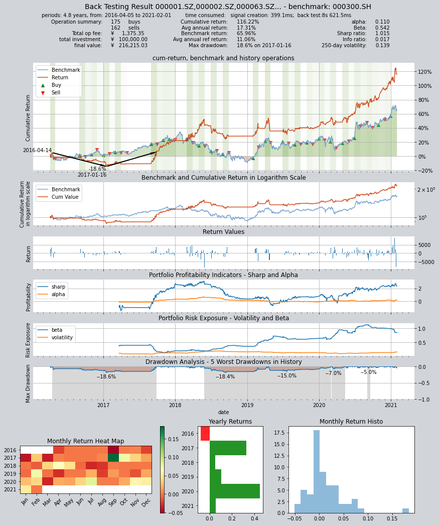
Results are as follows:
         ====================================
         |                                  |
         |       BACK TESTING RESULT        |
         |                                  |
         ====================================

    qteasy running mode: 1 - History back testing
    time consumption for operate signal creation: 0.0ms
    time consumption for operation back looping:  12s 766.3ms

    investment starts on      2016-04-05 00:00:00
    ends on                   2021-02-01 00:00:00
    Total looped periods:     4.8 years.

    -------------operation summary:------------
    Only non-empty shares are displayed, call
    "loop_result["oper_count"]" for complete operation summary

              Sell Cnt Buy Cnt Total Long pct Short pct Empty pct
    000001.SZ    1        1      2     1.7%      0.0%     98.3%
    000069.SZ    2        2      4     3.4%      0.0%     96.6%
    000301.SZ    3        3      6    13.6%      0.0%     86.4%
    000333.SZ    1        1      2     1.7%      0.0%     98.3%
    000338.SZ    1        1      2     3.5%      0.0%     96.5%
    000596.SZ    1        1      2     1.8%      0.0%     98.2%
    000651.SZ    1        1      2     1.7%      0.0%     98.3%
    000776.SZ    1        1      2     1.7%      0.0%     98.3%
    000786.SZ    1        1      2     1.7%      0.0%     98.3%
    000800.SZ    2        2      4     5.4%      0.0%     94.6%
    ...            ...     ...   ...      ...       ...       ...
    603806.SH    2        2      4     3.6%      0.0%     96.4%
    603939.SH    0        1      1     3.7%      0.0%     96.3%
    688599.SH    0        1      1     3.7%      0.0%     96.3%
    000408.SZ    1        1      2     1.7%      0.0%     98.3%
    002648.SZ    2        2      4     3.4%      0.0%     96.6%
    300751.SZ    1        1      2     1.7%      0.0%     98.3%
    688065.SH    1        1      2     1.7%      0.0%     98.3%
    600674.SH    2        2      4     3.7%      0.0%     96.3%
    600803.SH    1        1      2     1.7%      0.0%     98.3%
    601615.SH    1        1      2     1.7%      0.0%     98.3%

    Total operation fee:     ¥    1,290.37
    total investment amount: ¥  100,000.00
    final value:              ¥  216,271.60
    Total return:                   116.27%
    Avg Yearly return:               17.32%
    Skewness:                          0.29
    Kurtosis:                          7.52
    Benchmark return:                65.96%
    Benchmark Yearly return:         11.06%

    ------strategy loop_results indicators------
    alpha:                            0.115
    Beta:                             0.525
    Sharp ratio:                      0.956
    Info ratio:                       0.017
    250 day volatility:               0.149
    Max drawdown:                    18.93%
        peak / valley:        2018-05-25 / 2018-09-11
        recovered on:         2019-04-18

    ===========END OF REPORT=============
3.2. The second method for setting custom strategies involves using PT trading signals to set position targets:
After completing the calculation of stock selection factors, directly set the position target for each stock. This way, there is no need to know the position data, and the position target signal can be output directly. During the backtest process, trading signals are generated based on the actual position.
>>> class GroupPT(qt.GeneralStg):
...
...     def realize(self):
...
...         # 读取策略参数(开盘价大于收盘价的天数)
...
...         # 读取策略参数(开盘价大于收盘价的天数)
...         n_day = self.get_pars('n_day')
...
...         # 从历史数据编码中读取四种历史数据的最新数值
...         opens, closes = self.get_data('open_E_d', 'close_E_d')  # 从前一交易日起前30天内开盘价
...         opens = opens[-30:]
...         closes = closes[-30:]
...
...         # 选股因子为开盘价大于收盘价的天数,使用astype将True/False结果改为1/0,便于加总
...         factors = ((opens - closes) > 0).astype('float')
...         # 所有开盘价-收盘价>0的结果会被转化为1,其余结果转化为0,因此可以用sum得到开盘价大于收盘价的天数
...         factors = factors.sum(axis=0)
...         # import pdb; pdb.set_trace()
...         # 选出开盘价大于收盘价天数大于十天的所有股票的序号
...         all_args = np.arange(len(factors))
...         selected = np.where(factors > n_day)[0]
...         not_selected = np.setdiff1d(all_args, selected)
...         # 计算选出的股票的数量
...         selected_count = len(selected)
...         print(f'now {selected_count} shares are selected!')
...
...         # 开始生成交易信号
...         signal = np.zeros_like(factors)
...         if selected_count == 0:
...             return signal
...         # 所有被选中的股票均设置为正持仓目标
...         signal[selected] = 1. / selected_count
...         # 未被选中的股票持仓目标被设置为0
...         signal[not_selected] = 0
...
...         return signal
Create an Operator object and start backtesting the trading strategy
>>> alpha = GroupPT(name='GroupPS',
...                 description='本策略每隔1个月定时触发, 从SHSE.000300成份股中选择过去30天内开盘价大于前收盘价的天数大于10天的股票买入',
...                 pars=[Parameter((3, 25), par_type='int', name='n_day', value=10)],
...                 data_types=[StgData('open', freq='d', asset_type='E', window_length=32),
...                             StgData('close', freq='d', asset_type='E', window_length=32)],
...                )
>>> op = qt.Operator(alpha, signal_type='PT', run_freq='ME')
>>> op.set_parameter(0, par_values=(20,))
>>> qt.run(op=op, mode=1,
...        asset_type='E',
...        asset_pool=shares,
...        invest_start='20160405',
...        invest_end='20210201',
...        trade_batch_size=100,
...        sell_batch_size=1,
...        trade_log=True)
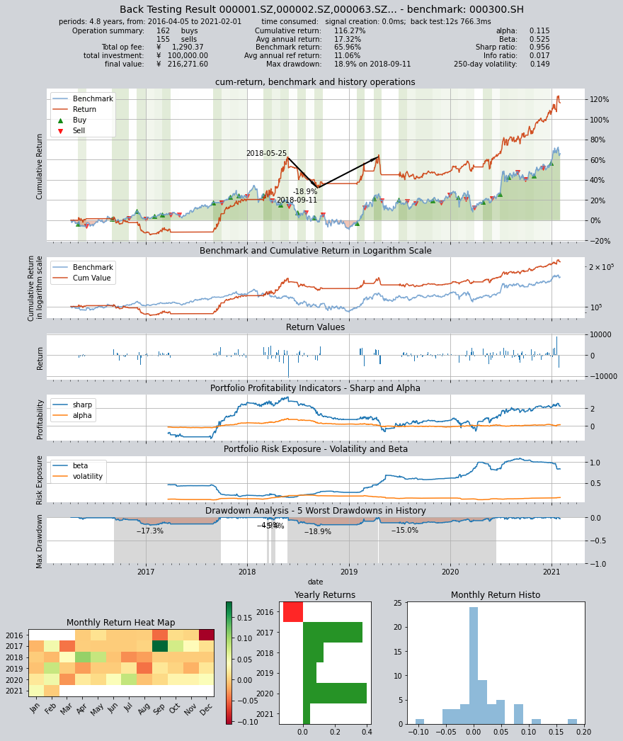
Results of the trading backtest are as follows:
         ====================================
         |                                  |
         |       BACK TESTING RESULT        |
         |                                  |
         ====================================

    qteasy running mode: 1 - History back testing
    time consumption for operate signal creation: 399.1ms
    time consumption for operation back looping:  8s 621.5ms

    investment starts on      2016-04-05 00:00:00
    ends on                   2021-02-01 00:00:00
    Total looped periods:     4.8 years.

    -------------operation summary:------------
    Only non-empty shares are displayed, call
    "loop_result["oper_count"]" for complete operation summary

              Sell Cnt Buy Cnt Total Long pct Short pct Empty pct
    000001.SZ    1        1       2    1.7%      0.0%     98.3%
    000069.SZ    2        2       4    3.4%      0.0%     96.6%
    000301.SZ    6        5      11   13.6%      0.0%     86.4%
    000338.SZ    1        1       2    1.7%      0.0%     98.3%
    000596.SZ    1        1       2    1.8%      0.0%     98.2%
    000625.SZ    1        1       2    1.7%      0.0%     98.3%
    000661.SZ    1        1       2    1.7%      0.0%     98.3%
    000776.SZ    1        1       2    1.7%      0.0%     98.3%
    000786.SZ    1        1       2    1.7%      0.0%     98.3%
    000800.SZ    2        3       5    5.4%      0.0%     94.6%
    ...            ...     ...   ...      ...       ...       ...
    603806.SH    2        2       4    3.6%      0.0%     96.4%
    603939.SH    0        2       2    3.7%      0.0%     96.3%
    688599.SH    0        2       2    3.7%      0.0%     96.3%
    000408.SZ    1        1       2    1.7%      0.0%     98.3%
    002648.SZ    1        1       2    1.7%      0.0%     98.3%
    300751.SZ    1        1       2    1.7%      0.0%     98.3%
    688065.SH    1        1       2    1.7%      0.0%     98.3%
    600674.SH    2        2       4    3.7%      0.0%     96.3%
    600803.SH    1        1       2    1.7%      0.0%     98.3%
    601615.SH    1        1       2    1.7%      0.0%     98.3%

    Total operation fee:     ¥    1,375.35
    total investment amount: ¥  100,000.00
    final value:              ¥  216,215.03
    Total return:                   116.22%
    Avg Yearly return:               17.31%
    Skewness:                          0.23
    Kurtosis:                          6.63
    Benchmark return:                65.96%
    Benchmark Yearly return:         11.06%

    ------strategy loop_results indicators------
    alpha:                            0.110
    Beta:                             0.542
    Sharp ratio:                      1.015
    Info ratio:                       0.017
    250 day volatility:               0.139
    Max drawdown:                    18.58%
        peak / valley:        2016-04-14 / 2017-01-16
        recovered on:         2017-09-27

    ===========END OF REPORT=============