7. Build your first strategy
qteasy is a fully localized deployment and operation of quantitative trading analysis toolkit, with the following functions:
Aquire, clean, store, process, visualize and use financial data
Create quantitative trading strategies, and provide a large number of built-in basic trading strategies
Vectorized high-speed trading strategy backtesting and trading result evaluation
Optimization and evaluation of trading strategy parameters
Deployment and real-time operation of trading strategies
You will understand the basic functions and usage of qteasy through a series of practical examples in this series of tutorials.
7.1. Before you start
Please make sure you have mastered the following content before starting this tutorial:
Install and upgrade
qteasyto the latest version, and complete the initialization configuration ofqteasyPrepare the local data source, master the method of downloading various financial data, and be able to download various historical price data, financial statement data, etc. of indexes and stocks to the local.
In the previous tutorial, I explained how to configure a local data source, search for and download financial data locally, and extract data from the local data source. If you haven’t completed this step yet, please refer to the previous tutorial to learn how to download and work with the data.
7.2. Target of this chapter
We will test a large-cap and small-cap rotation trading strategy through the creation of the qteasy module in this chapter.
The large-small cap rotation is a very basic and common trading strategy. This trading strategy captures the characteristics of the asynchronous rise and fall of large-cap stocks and small-cap stocks, and alternately holds large-cap stocks and small-cap stocks in the hope of obtaining higher returns. By creating this trading strategy, we can easily understand how to use qteasy to create trading strategies, call historical price backtesting trading strategies, analyze the performance of strategies, and improve strategies.
Now, we need to create the simplest rotation strategy: rotate between the two indices mentioned earlier, and hold the index with the larger possible increase in the future every day:
Calculate the increase of the two indices in the past 20 days, that is, the increase of today’s price relative to the price 20 days ago
Choose the index with the larger increase, hold it the next day, and sell the index with the smaller increase
7.3. Realize the strategy
According to the above strategy idea, we can easily implement such a rotation stock selection strategy in qteasy, because qteasy has built-in nearly 70 trading strategies, all built-in strategies have unique names, and these built-in strategies can be used directly by referencing the names. All trading strategies in qteasy must be included in an object named Operator, which is actually a container for strategies. It can be understood that a trader can manage multiple strategies at the same time and run these strategies at the same time to generate trading signals.
An Operator object can be created directly through qt.Operator(), and the strategies parameter can be passed when creating to create trading strategies at the same time:
>>> import qteasy as qt
>>> op = qt.Operator(
...     strategies = 'ndayrate',  # 创建交易员对象时,同时创建一个交易策略“ndayrate”
...     run_freq='d',   # 交易策略的运行频率为每天运行一次
...     run_timing='close',  # 交易策略的运行时机为每天股票收盘时运行
... )
With the code above, we have already created a single-factor stock-selection strategy (ndayrate) in qteasy. This strategy is a built-in stock-selection strategy: it selects stocks based on the “N-day price increase.” Its selection logic is to evaluate the N-day price increase of all stocks in the stock pool, and then select stocks or assets based on that price increase (of course, the selection method is configured via parameters, which will be mentioned below).
With the qt.built_ins() function, you can view detailed descriptions of built-in strategies:
>>> qt.built_in_doc('ndayrate', print_out=True)
The output is as follows:
以股票过去N天的价格或数据指标的变动比例作为选股因子选股
    基础选股策略:根据股票以前n天的股价变动比例作为选股因子

    策略参数:
        n: int, 股票历史数据的选择期
    信号类型:
        PT型: 百分比持仓比例信号
    信号规则:
        在每个选股周期使用过去N日内价格变动率作为选股因子进行选股
        通过以下策略属性控制选股方法:
        - max_sel_count:     float,  选股限额,表示最多选出的股票的数量,默认值: 0.5,表示选中50%的股票
        - condition:         str ,   确定股票的筛选条件,默认值any
            - any        :默认值,选择所有可用股票
            - greater    :筛选出因子大于ubound的股票
            - less       :筛选出因子小于lbound的股票
            - between    :筛选出因子介于lbound与ubound之间的股票
            - not_between:筛选出因子不在lbound与ubound之间的股票
        - lbound:            float,  执行条件筛选时的指标下界, 默认值np.-inf
        - ubound:            float,  执行条件筛选时的指标上界, 默认值np.inf
        - sort_ascending:    bool,   排序方法,默认值: False,
            - True: 优先选择因子最小的股票,
            - False, 优先选择因子最大的股票
        - weighting:         str ,   确定如何分配选中股票的权重,默认值: even
            - even       :所有被选中的股票都获得同样的权重
            - linear     :权重根据因子排序线性分配
            - distance   :股票的权重与他们的指标与最低之间的差值(距离)成比例
            - proportion :权重与股票的因子分值成正比
    策略属性缺省值:
        默认参数: (14,)
        数据类型: close 收盘价,单数据输入
        窗口长度: 150
        参数范围: [(2, 150)]
    策略不支持参考数据,不支持交易数据
Now, an Operator object and a trading strategy have been created.
We can use Operator.info() to view detailed information about the trader object and the trading strategies. Meanwhile, we can access all trading strategies via the Operator.strategies attribute.
>>> op.info()
>>> stg = op.strategies[0]  # 获取op的第一个策略,下面的几种方法是等效的
>>> # stg = op[0]
>>> # stg = op['ndayrate']
>>> # stg = op.get_strategy_by_id('ndayrate')
The output is as follows:
==============================Operator Information==============================
Name:        None
Run Mode:    batch - All history operation signals are generated before back testing
Groups:      1 Strategy(s) in 1 Group(s)

------------------------------------Group_1-------------------------------------
Signal Type: pt - Position Target, signal represents position holdings in percentage of total value
Run Timing:  close @ d - days
Strategies (1): ['ndayrate']
Signal blenders: ndayrate

------------------------------Strategies in group-------------------------------
stg_id          name                    parameters
--------------------------------------------------------------------------------
ndayrate        N-DAY RATE              (14,)
================================================================================
You can also view more detailed strategy parameters and information via the trading strategy’s info() method:
>>> stg.info()
Output as follows
============================= Strategy: N-DAY RATE =============================
Strategy FACTOR(N-DAY RATE)
Parameters: ['n'] = (14,)
Date Types: close_ANY_d x 150
----------------------------- Selection Properties -----------------------------
Max select count        50.0%
Sort Ascending          False
Weighting               even
Filter Condition        any
Filter ubound           inf
Filter lbound           -inf
We can see from the above information that the ndayrate strategy has many configurable parameters. By adjusting these parameters, we can adjust the stock selection method of the strategy, thereby adjusting the performance of the trading strategy.
Now, we need to make some basic settings to ensure that this stock selection strategy selects stocks as we want. All parameters in the Operator object can be implemented through the op.set_parameter() method.
>>> op.set_parameter(0,   # 指定需要设置参数的交易策略:即设置策略0的参数
...                  sort_ascending=False,  # 设置选择涨幅最大的指数
...                  max_sel_count=1,  # 设置选股数量,每次最多从投资池里选择一支股票
...                  par_values=(20, ),  # 策略参数N=20,比较20日涨幅
...                  data_types=[qt.StgData('close',  # 使用收盘价计算涨幅
                                            freq='d',  # 使用每日收盘价
                                            asset_type='ANY',  # 适用于任何类型的资产
                                            use_latest_data_cycle=True,  # 使用最新的数据周期,每次选股数据包括当天收盘价在内
                                            window_length=25,  # 数据窗口长度为25天
                                            )],
... )
In above code snippet, we set the basic behavior of the stock selection strategy through several simple parameter settings:
sort_ascending=False: Sort order: This strategy sorts the selection metric and takes the top entries. Because it needs the largest return, it should be sorted in descending order. If you want the smallest return, setsort_ascending=True.max_sel_count=1: Number of selected securities: This parameter controls the number of securities selected. Since it always chooses one out of two indices, this parameter is set to 1.par_values=(20, ): Strategy parameter values: This strategy uses a tunable parameter N, meaning it selects securities based on the N-day return. Setting it to 20 means using the 20-day price return as the selection factor.data_types=[qt.StgData(...)]: Data types: Determines what data the strategy uses to calculate the selection factor. Here, a StgData object is used, which contains the following parameters:freq='d': Here we use the closing price to calculate price returns, and set the window length to 25, so each time the strategy runs, it will read the current day as well asasset_type='ANY': Asset type: This strategy applies to any type of asset. Of course, it can also be set to a specific asset type, such as stocks, indices, funds, etc.use_latest_data_cycle=True: Data cycle: This parameter controls the data cycle used each time the strategy runs. Setting it to True means using the latest data cycle—i.e., each stock selection includes that day’s closing price. If set to False, the data seen by each strategy run does not include that day’s closing price. In real operation, it’s actually impossible to trade using the exact closing price of the day, because you can’t trade after the market closes. However, we can trade using the real-time price one minute before the close; this price is usually very close to the closing price. Here, using the day’s closing price is a simplified backtesting approach.window_length=25: data window length. qteasy ensures that each time the strategy runs, it can only see data from a period looking back from the current run time, thereby avoiding look-ahead bias. Setting it to 25 means that each time you select stocks, you can only see the 25 prices from 25 days ago up to the current day, ensuring there is enough data when calculating the 20-day return.
Prepare backtest data
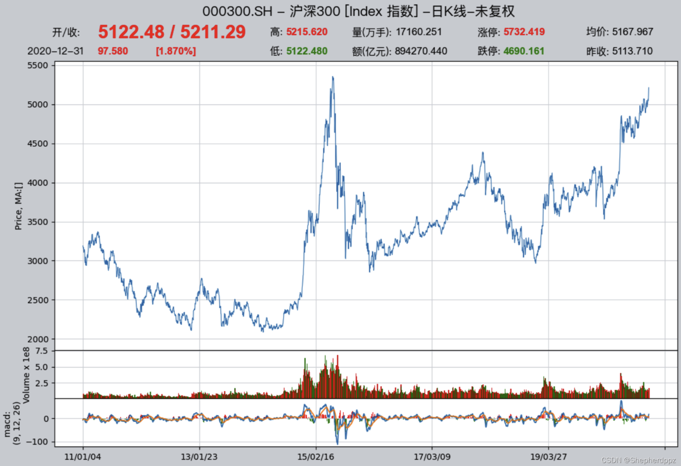
After configuring the stock selection strategy, it is necessary to verify the performance of the strategy through backtesting, that is, call the actual historical data of the Shanghai and Shenzhen 300 and ChiNext two indices, conduct simulated trading, and see if the results of simulated trading can outperform the market. In actual operation, it is not easy to buy and sell large-cap indices, but it is generally easy to find ETF funds that track large-cap indices to replace large-cap indices. For simplicity, we will invest in the Shanghai and Shenzhen 300 and ChiNext indices from January 1, 2011 to December 31, 2020, assuming a transaction fee rate of one thousandth, and see how the investment results are.
Previously, we have learned how to download historical data. Here we need all the data of the Shanghai and Shenzhen 300 and ChiNext indices from 2013 to the end of 2022.
Note When downloading historical data for backtesting, the downloaded data needs to be more than the starting point of the backtesting date. For example, if the backtesting starts on January 1, 2013, more data is actually needed, so the starting point of the downloaded data should start from September 2012. For a detailed analysis of this, please refer to the reference document
Download the corresponding historical data using the following code:
>>> qt.refill_data_source(tables='index_daily', symbols='399006, 000300', start_date='20100901', end_date='20201231')
Confirm whether the data is downloaded successfully:
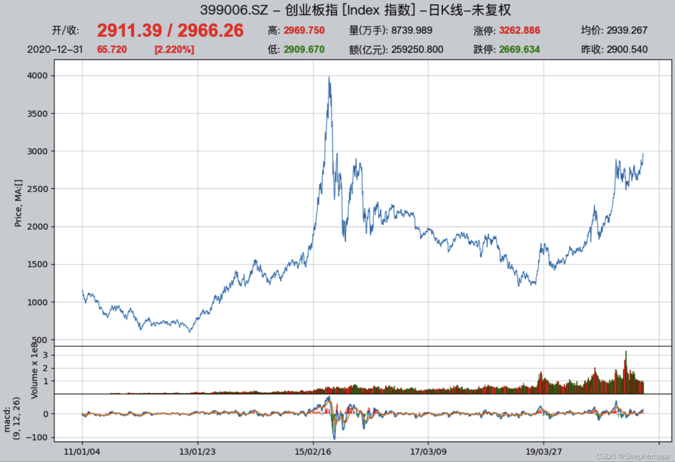
>>> qt.candle('000300.SH', start='20110101', end='20201231', asset_type='IDX', mav=[])
>>> qt.candle('399001.SZ', start='20110101', end='20201231', asset_type='IDX', mav=[])
Configure backtest parameters
After the data is ready, you can start configuring the backtest parameters and start backtesting. The strategy backtesting of qteasy is completely parameterized. Before backtesting, we need to tell the system all relevant information, such as the variety of investment products, the amount of funds invested, the start and end dates of backtesting, the transaction fee calculation method during backtesting, and the transaction batch, etc. We can use qt.configure() to configure the backtest parameters:
>>> qt.configure(asset_pool=['000300.SH',
...                          '399006.SZ'],  # 投资股票池里包括沪深300和创业板指数两个指数,分别代表大盘和小盘股
...              invest_cash_amounts=[100000],  # 投入金额为十万元
...              asset_type='IDX',  # 为简单起见,直接投资于指数
...              cost_rate_buy=0.0001,  # 买入资产时交易费用万分之一
...              cost_rate_sell=0.0001,  # 卖出资产时的交易费用为万分之一
...              invest_start='20110101',  # 模拟交易开始日期
...              invest_end='20201231',  # 模拟交易结束日期
...              trade_batch_size=0.01,  # 买入资产时最小交易批量
...              sell_batch_size=0.01,  # 卖出资产时最小交易批量
... )
The meaning of the above configuration is as follows
asset_pool=['000300.SH', '399006.SZ']:Investment target index is given in list form. If you want to invest in other indexes or ETF funds, you can directly pass in the security code. If you want to select stocks from three or more securities, you can directly add them to the list.invest_amounts=100000:The investment amount is one hundred thousand yuan. If you need to simulate multiple batch investments, you can also pass in a list, but you need to specify the specific date of each investment separately.asset_type='IDX':Investment target type:'E'represents stocks,'IDX'represents indexes,'FD'represents funds,'FT'represents futures,'OPT'represents optionscost_rate_buy=0.0001:Set the buy and sell transaction fee ratio.qteasyalso supports setting the minimum fee, fixed fee, etc. Here, only the fee rate needs to be set.cost_rate_sell=0.0001:invest_start='20110101':Simulation trading start dateinvest_end='20201231':Simulation trading end datetrade_batch_size=0.01: the minimum trading lot size when buying assets; the minimum allowed is0.01. A value of 1 means you can only trade whole shares/units; here you can enter any number greater than or equal to0.01.sell_batch_size=0.01: the minimum trading lot size when selling assets; the minimum allowed is0.01.
qteasy还有其他的配置参数,参见QTEASY文档。
7.4. Results of backtesting the strategy
It is very simple to backtest the strategy of qteasy. After setting all the configurations, you can start backtesting. You can call qt.run() to start backtesting. At the same time, we enable visual chart output and open trading details recording:
>>> res = qt.run(op, mode=1, visual=True, trade_log=True) # 调用qteasy的run方法,启动回测交易
After waiting a moment, the backtest completes, and qteasy will print the backtest report to the terminal.
The output is as follows:
In the report, you can directly see a comparison between our total investment return and the return of the CSI 300 Index over the same period:
====================================
|                                  |
|         BACKTEST REPORT          |
|                                  |
====================================
qteasy running mode: 1 - History back testing
... 内容略,详见下文报告解析
-------------operation summary:------------
... 内容略,详见下文报告解析

Total operation fee:      ¥   10,666.34
total investment amount:  ¥  100,000.00  # 投入的总金额为十万元
final value:              ¥  611,231.20  # 回测结束时的资产总额
Total return:                   511.23%  # 投资的总收益率
Avg Yearly return:               19.86%  # 投资的年化收益率为19.86%
... 内容略,详见下文报告解析
Benchmark return:                60.32%  # 同期沪深300指数的总回报率为60.32%
Benchmark Yearly return:          4.84%  # 同期沪深300指数的年化收益率仅有4.84%

------strategy loop_results indicators------
... 内容略,详见下文报告解析

==================END OF REPORT===================
From the backtest results, it is easy to see that this strategy outperformed the CSI 300 benchmark index. Over these ten years, the CSI 300’s annualized return was only a paltry ~5% (4.84%), even worse than some higher-yield fixed-term products, while our strategy’s annualized investment return reached 19.86%. Over ten years, total assets grew from 100,000 yuan to more than 600,000 yuan—more than a sixfold increase.
7.5. Improvement of the strategy
Our strategy somewhat successful. However, just looking at the total return rate cannot fully explain the problem. How does the strategy perform throughout the ten years? This requires further analysis to see if the strategy can be further improved. At this time, we need to further check the results of the backtest, especially the visual results and trading details records, to find the shortcomings and improvement points of the strategy through these records and reports.
To further improve, we need to analyze the strategy’s performance in greater depth, identify its shortcomings, and find directions for improvement. To this end, qteasy provides the following tools to help users analyze backtest results:
Backtest report: you need to set
report=True. The backtest report summarizes the backtest results in text form, making it easy to quickly grasp the investment return and key evaluation metrics.Visual report: set
visual=True. A visual composite chart presents the contents of the backtest report in graphical form and provides more detailed information, making it easier for users to understand the backtest results more intuitively.Trade log file: Requires setting:
trade_log=True. The trade log file records every strategy run during the backtest in the form of a CSV file, including key variables of the strategy run and the stock selection results each time. This makes it easier for users to analyze how the strategy runs, identify its shortcomings, and find directions for improvement.Trade detail report: set
trade_log=True. The trade detail report records detailed information for each trade in a CSV file, making it easier for users to analyze the details of each trade, identify the strategy’s shortcomings, and find directions for improvement.
Next, we will take a detailed look at the content and usage of each tool to help us analyze backtest results, identify the strategy’s shortcomings, and find directions for improvement.
Detailed explanation of the backtest report:
The backtest report of qteasy contains a large amount of statistical information about backtest results. Let’s go through it in detail one by one:
Part 1: Basic backtest information
The first part of the report contains the basic information of the backtest, including the time taken, the start and end dates, the total backtest period, and so on. This information helps us understand the basics of the backtest:
qteasy running mode: 1 - History back testing
time consumption for operate signal creation: 123.2 ms  # 生成交易信号的时间
time consumption for operation back testing:  288.7 ms  # 回测交易的时间
investment starts on      2011-01-04 15:00:00           # 回测开始日期
ends on                   2020-12-30 15:00:00           # 回测结束日期
Total looped periods:     10.0 years.                   # 回测的总周期为十年
Part 2: Trading operation statistics
The second part of the backtest report is trading operation statistics. In list form, it counts the number of buys and sells for each investment instrument, as well as the proportion of time it was held:
For example, we can see that 000300.SH (CSI 300 Index) was bought 75 times and sold 81 times over ten years, with a position-holding time ratio of 47.7% and a cash (out-of-market) time ratio of 52.3%; whereas 399006.SZ (ChiNext Index) was bought 105 times and sold 85 times over ten years, with a position-holding time ratio of 47.9% and a cash (out-of-market) time ratio of 52.1%.
-------------operation summary:------------
Only non-empty shares are displayed, call
"loop_result["oper_count"]" for complete operation summary
          Sell Cnt Buy Cnt Total Long pct Short pct Empty pct
000300.SH   101       97    198   50.4%     -0.0%     49.6%
399006.SZ   102      101    203   50.2%     -0.0%     49.8%
Part 3: Backtest result statistics
The third part of the backtest report is backtest result statistics, including important metrics such as the total amount invested, final total assets, total return, annualized return, benchmark return, and more:
Total operation fee:      ¥   10,666.34  # 投资过程中的总交易费用
total investment amount:  ¥  100,000.00  # 投入的总金额
final value:              ¥  611,231.20  # 回测结束时的资产总额
Total return:                   511.23%  # 投资的总收益率
Avg Yearly return:               19.86%  # 投资的年化收益率
Skewness:                         -0.40  # 投资回报率的偏度,偏度表明投资回报率分布的偏斜程度,负偏度表明投资回报率分布的左尾较长,意味着投资回报率有较大的负面极端值的可能性
Kurtosis:                          2.79  # 投资回报率的峰度,峰度表明投资回报率分布的峰态程度,峰度越大,表明投资回报率分布的峰态越高,意味着投资回报率有较大的极端值的可能性
Benchmark return:                60.32%  # 基准收益率,这里是指投资标的的基准指数(默认沪深300指数)的收益率,该指数在同一时段内收益率只有60%
Benchmark Yearly return:          4.84%  # 基准年化收益率,这里是指投资标的的基准指数(默认沪深300指数)的年化收益率,该指数在同一时段内年化收益率只有4.84%
Part 4: Strategy performance metrics
The fourth part of the backtest report is strategy performance metrics, including important indicators such as Alpha, Beta, Sharpe Ratio, Information Ratio, 250-day volatility, maximum drawdown, and so on.
------strategy loop_results indicators------
alpha:                            0.219  # 投资策略的Alpha值,Alpha值表明投资策略相对于基准指数的超额收益率,Alpha值越大,表明投资策略相对于基准指数的表现越好
Beta:                             0.686  # 投资策略的Beta值,Beta值表明投资策略相对于基准指数的系统风险,Beta值越大,表明投资策略相对于基准指数的系统风险越大
Sharp ratio:                      0.880  # 投资策略的Sharp Ratio,Sharp Ratio表明投资策略的风险调整收益率,Sharp Ratio越大,表明投资策略的风险调整收益率越好
Info ratio:                       0.062  # 投资策略的Info Ratio,Info Ratio表明投资策略相对于基准指数的风险调整超额收益率,Info Ratio越大,表明投资策略相对于基准指数的风险调整超额收益率越好
250 day volatility:               0.265  # 投资策略的250日波动率,250日波动率表明投资策略在250个交易日内的收益率波动程度,250日波动率越大,表明投资策略的收益率波动程度越大
Max drawdown:                    48.25%  # 最大回撤,最大回撤表明投资策略在回测期间内的最大资产回撤程度,最大回撤越大,表明投资策略的风险越大
    peak / valley:        2015-06-03 / 2015-08-26  # 最大回撤从2015年6月3日的峰值开始,到2015年8月26日的2015年8月26日,投资收益达到回撤48.25%
    recovered on:         2020-02-21               # 从2015年8月26日开始反弹,一直到2020年2月21日才完全恢复到2015年6月3日的峰值水平,也就是说,最大回撤持续了近五年时间
Detailed explanation of the visual report
As long as you set the qteasy environment configuration variable visual=True, you can see a visual chart report of the results at the end of the backtest report:
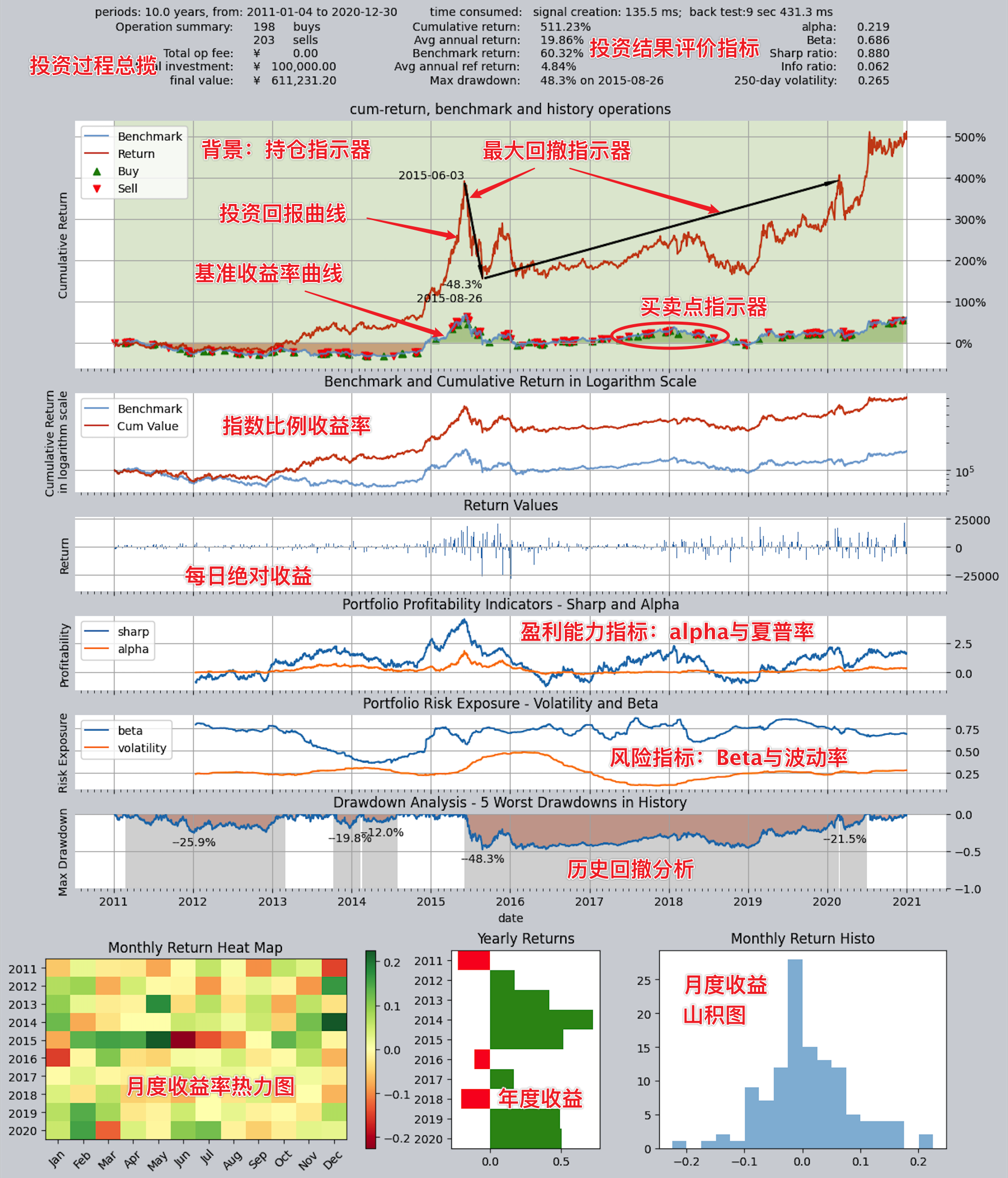
The visualization charts present all the information in the backtest report in a more intuitive way using composite charts. As you can see, the main body of this chart includes six historical line charts sharing a unified time axis, and below are three side-by-side bar charts that summarize annual and monthly returns.
Overall, this chart can be divided into four parts. Let’s go through them one by one:
Part 1: Basic information and investment return metrics
At the very top of the chart, it shows the basic backtest information and return metrics. This information is basically consistent with what’s in the backtest report, including important return metrics such as the investment’s total return, annualized return, and the benchmark index’s return, helping users quickly understand the investment’s performance.
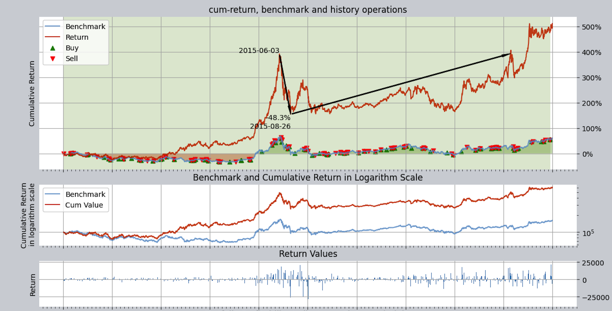
Part 2: Return Curve Chart
The backtest historical return curve section includes three charts. They all show historical returns, but each has a different focus.
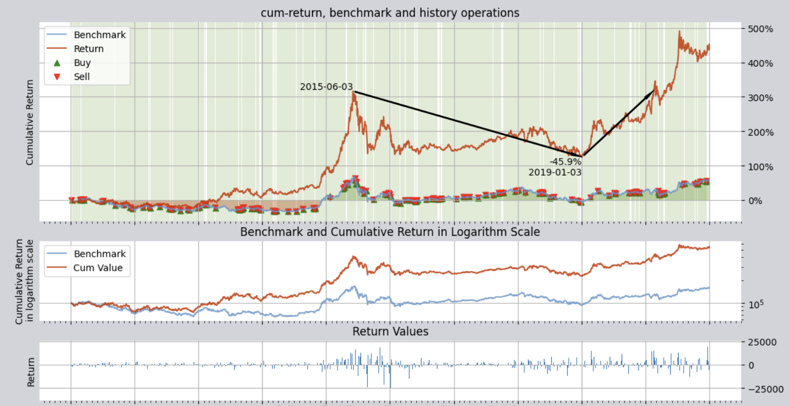
The three charts are:
Return Curve: This curve chart uses percentages and records the historical return curves of investment returns and benchmark returns with two lines (by default, the benchmark is the CSI 300 Index; you can set other indices via the environment configuration variable
reference_asset). The red curve represents the portfolio return, while the blue curve represents the reference index return. This chart includes some additional information that can be enabled or disabled via environment variables:Drawdown indicator: uses black arrows to mark the peak, trough, and recovery date of the single largest drawdown within the investment period, making it easier for users to understand the investment’s maximum drawdown.
Buy/sell indicator (set
buy_sell_points=True): on the green line representing the benchmark return curve, each buy and sell is marked with a red/green arrow at the corresponding time point. Red indicatesPosition indicator (set
show_positions=True): the chart background uses light vertical stripes to indicate the position ratio for each period. Green represents a long position, and red represents a short position (the figure above has only long positions, no short positions). The darker the stripe color, the higher the position ratio; conversely, it indicates a lower position ratio.
Log Return Curve: This curve chart uses log returns as the unit and shows the historical curves of investment returns and benchmark returns. The log return curve can better show the trend of changes in investment returns, especially when returns are relatively high or low, making changes in returns clearer.
Return Bar Chart: This chart uses bars to show the daily profit/loss amount within the backtest historical period.
From the return curve chart, you can see that although the overall returns are fairly good, the drawdown is relatively high, with a maximum of 45%.
You can imagine that if an investor started investing on June 3, 2015, the result would be: a 45.9% loss by January 3, 2019, and they wouldn’t break even until after 2020!
Part 3: Performance metric curve chart
The third part of the charts is the strategy performance metrics section, mainly used to evaluate the strategy’s profitability and risk control capability. It also includes three charts:
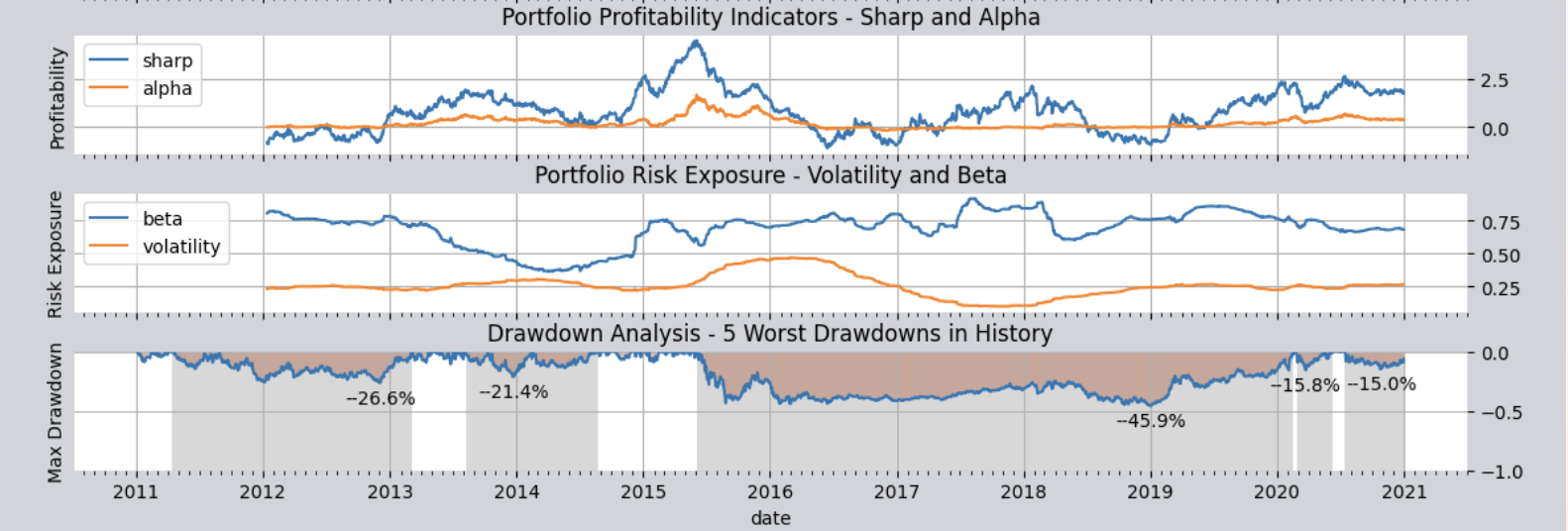
Profitability metrics: The first chart shows the metrics used to evaluate the strategy’s profitability, displaying the historical rolling values of two indicators: the Sharpe ratio and alpha. Both indicators are widely used to evaluate a trading strategy’s ability to generate excess profits (i.e., above the benchmark). Each point on the two lines in the chart is the rolling Sharpe ratio and alpha calculated over the past 250 trading days ending on that day, so you can see how these two lines change over time. The higher the Sharpe ratio, the better the strategy’s risk-adjusted return; the higher the alpha, the better the strategy’s excess return relative to the benchmark index.
Risk control capability metrics: The second chart shows the metrics used to evaluate the strategy’s risk control capability, displaying the historical rolling values of two indicators: beta and volatility. Both indicators assess whether the strategy can control risk. The lower the beta, the smaller the strategy’s systematic risk relative to the benchmark index; the lower the volatility, the smaller the fluctuation in the strategy’s returns.
Drawdown control capability metric: The third chart is the drawdown underwater chart, showing the evaluation metric of the strategy’s drawdown control capability. It displays the historical curve of the investment return rate and the historical drawdown curve of the investment return rate (i.e., the “underwater” curve). Each dip in this curve indicates that the investment return curve has drawn down relative to a previous high; the deeper the dip, the more severe the drawdown. One complete dive and resurfacing represents one complete drawdown cycle. At the same time, this chart uses gray bars to mark the five deepest drawdown periods in history; the wider the gray bar, the longer the drawdown lasted.
From the drawdown underwater chart, you can see that over the entire ten-year period, except for a brief one or two years, it was almost always in an underwater, trapped state, and the maximum underwater depth reached more than 45%. Throughout the ten-year investment period, total assets kept experiencing drawdowns; the 45% drawdown was the largest and deepest one, but earlier there were also multiple drawdowns such as 26% and 22%, and none of them were short. The whole investment was basically “being trapped for the long term, with occasional chances to recover.” I believe very few investors could endure that kind of ordeal, right?
Part 4: Return statistics chart
At the very bottom there are three charts side by side, which summarize annual or monthly returns from different perspectives:
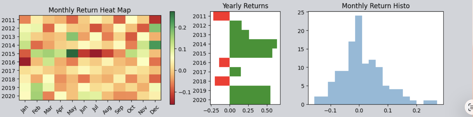
Monthly Return Heatmap: Displays returns for each month (x-axis) across years (y-axis) in colored blocks. The greener the color, the higher the return; the redder the color, the lower the return or the greater the loss.
Annual Return Bar Chart: Intuitively shows the return for each year. Green bars indicate positive returns, red bars indicate losses; the taller the bar, the larger the absolute value of the gain/loss.
Monthly return histogram: It counts the returns for all months and plots their probability distribution. Overall, this chart usually resembles a bell curve similar to a normal distribution. However, depending on the strategy’s performance, the bell curve may shift to the right as a whole, indicating a higher overall probability of generating positive returns, or it may become skewed, helping users statistically understand the distribution of returns.
From the three charts above, you can see that over the entire decade there were three years (2011, 2016, and 2018) with negative returns, while all other years achieved positive returns. However, the returns fluctuate greatly: some years make big profits, while others suffer big losses. Large fluctuations indicate that the strategy carries high risk and has relatively weak risk control.
At this point, by analyzing the charts, we now have a very intuitive understanding of the trading strategy’s overall returns: the biggest problem with this strategy is that it did not control drawdowns well.
Therefore, we should find ways to improve this strategy and see how we can reduce drawdowns and enhance performance. To do so, we need to carefully analyze every trade during the simulated trading backtest process to find ways to reduce drawdowns. To view every detail of the backtest trades, you need to check the trade log files.
Next, we will continue with a detailed explanation of the trading log file.
Detailed Explanation of the Trading Log / Trading Report
As long as we set the environment variable trade_log=True, the system will generate multiple CSV files after each backtest (at least including the trade log and the trade detail report; in the current version, when this option is enabled it will also write the net value curve value_curve_*, etc.; refer to what is actually generated). The save path of these files is controlled by the configuration item trade_log_file_path, which defaults to QT_ROOT_PATH/tradelog/. This path supports relative paths, absolute paths, and home-directory paths starting with ~, and it can be modified at runtime via qt.configure(trade_log_file_path='...') and take effect immediately (hot update) without re-importing. For example:
On Windows, specify a directory on another drive:
qt.configure(trade_log_file_path='C:\\qt_trade_logs\\')On macOS/Linux, specify a directory under your home folder:
qt.configure(trade_log_file_path='~/qt_trade_logs/')
Disk retention policy: The configuration item trade_log_keep_days defaults to 3, meaning that after each time a new process imports qteasy it will clean up expired backtest CSV files under the trade_log_file_path directory according to this number of days, such as trade_log_*, trade_summary_*, and value_curve_* (it does not automatically clean up before writing files for each backtest). To keep all historical files long-term, set trade_log_keep_days to None or less than or equal to 0; you can also call qt.rotate_trade_logs(days=...) at any time to clean up manually.
If you want to view the current log file save path, please use:
import qteasy as qt
print(qt.QT_TRADE_LOG_PATH)
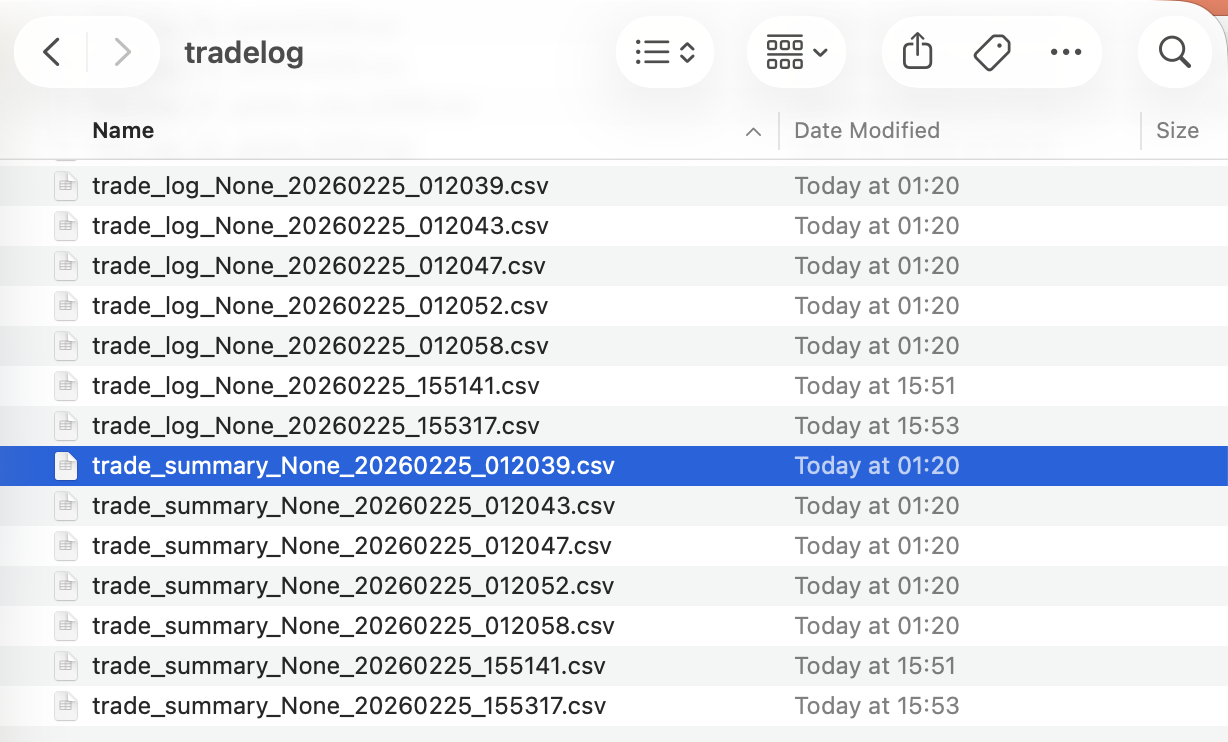
Open the folder at that path and you can see reports from each backtest. All reports are saved as CSV files for easy opening in Excel. Common types include:
Trade log: Files starting with “trade_log” are trade log files, listing detailed information for each strategy run.
Trade report: Files starting with “trade_summary” are trade reports, listing information for each trade.
Net value curve (if generated): Files starting with “value_curve” record the complete net value series, etc.
All of the above files end with the date/time of the backtest run to distinguish log files generated at different times. We explain them separately:
Interpreting the Trade Logs
Open the first file with Excel to see the trade log. The trade log records, in a table, information such as changes in funds for each strategy run, changes in positions, and trade details for each stock. Regardless of whether there are trades or position changes, there is a record every day:
The entire trading history is arranged by rows in the table, with every eight rows as one group. Each group records one trade, and the information from the first trade to the last is recorded in order from top to bottom.
The eight lines in each group of records respectively capture the following:
0, trade signal Trade signals: Records the trade signals generated after this run (trade signals are a set of numbers; after signal parsing they become trade orders. See Trade Signals for details).
1, price Trade price: Records the trading prices of each stock during this run.
2, traded amounts Traded quantity: Records the actual traded quantity for each stock after this run. Positive numbers indicate buy quantity, negative numbers indicate sell quantity, and 0 means no trade.
3, cash changed Cash change: Records the amount of cash change caused by actual trades for each stock after this run. Positive numbers indicate an increase in cash, negative numbers indicate a decrease in cash, and 0 means no change.
4, trade cost Transaction costs: Records the transaction costs actually incurred for each stock after this run.
5, own amounts Position size: Records the quantity held for each stock after this run. Positive numbers indicate long position size, negative numbers indicate short position size, and 0 means no position.
6, available amounts Available positions: Records the available quantity for each stock after this run. Positive numbers indicate available long position size, negative numbers indicate available short position size, and 0 means no available holdings.
7, summary Summary: Records the total held/available cash, total market value of holdings, and total portfolio value after this run.
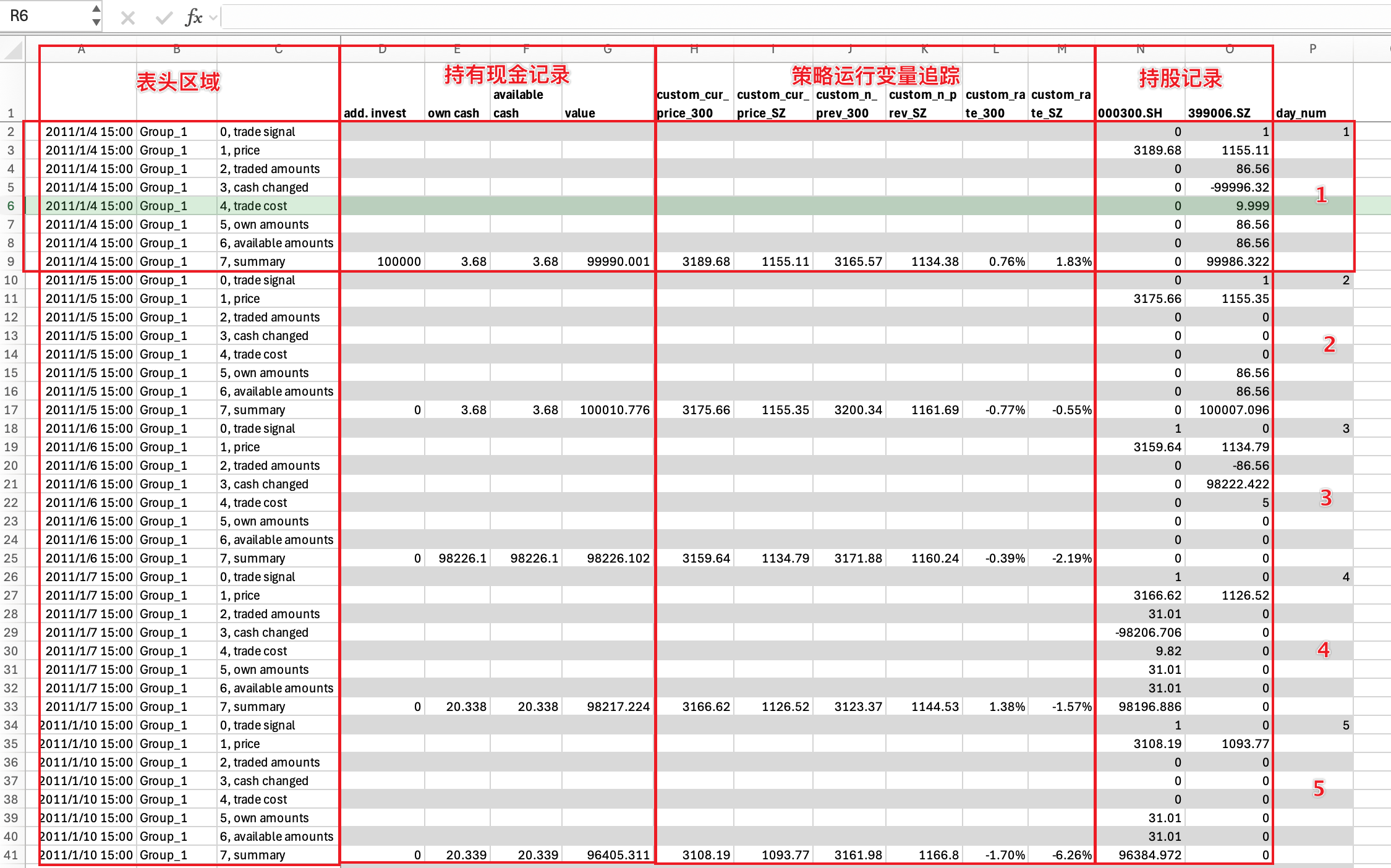 By examining the trade log closely, the entire table can be divided by columns into three or four groups, each providing information from a different perspective:
Header area: The first column in the header area records the date and time of each run, the second column records the strategy group name for each run (see Strategy Groups for details), and the third column labels the name of each row,
Cash holdings record: In the summary row of this area, it records the additional cash invested before each run, the total cash held at period end / total available cash, and the total portfolio value (including total cash and total stock market value).
Strategy Runtime Variable Tracking: Strategy runtime variable tracking is optional. It allows users to insert tracking points in the strategy to track the values of variables during strategy execution, which is very useful during strategy debugging. We will skip it for now; see details in
Holding Records: This area shows information such as the number of shares held, the number of shares traded, and the trading price for each stock in the investment stock pool. Each column shows the data for one stock, and the number of columns equals the number of stocks in the stock pool.
Based on the understanding above, we can analyze the strategy’s execution process and see how the strategy selects and rotates stocks.
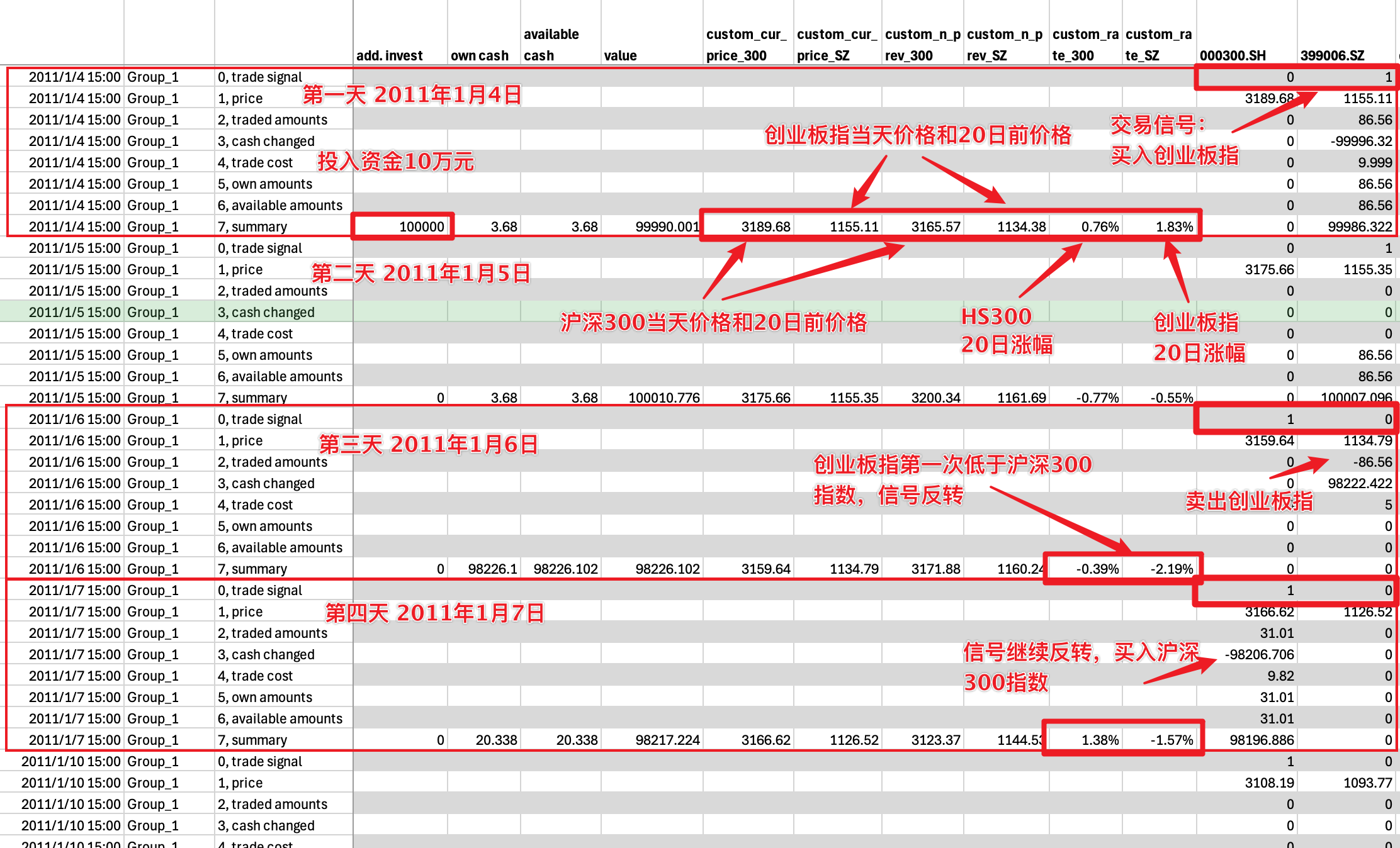
As shown above, we can use the run records from the first four days to gain a deeper understanding of how the strategy operates:
Day 1: An initial capital of 100,000 yuan was invested and the investment started. At the same time, we can see that the gains of the CSI 300 and the ChiNext Index that day were 0.76% and 1.83%, respectively. According to the strategy rules, we bought 86.56 shares of the ChiNext Index at the close, spending 99,996.32 yuan. After the trade, we held 86.56 shares of the ChiNext Index;
Day 2: The gains of the ChiNext Index and the CSI 300 Index were -0.77% and -0.56%, respectively. Comparing the two, the ChiNext Index still came out ahead, so the position remains unchanged;
Day 3: The CSI 300 Index’s gain surpassed that of the ChiNext Index. At this point, the trading signal reversed, generating both a CSI 300 buy signal and a ChiNext sell signal. However, only the ChiNext sell signal was executed: we sold all 86.56 shares. The CSI 300 buy signal could not be executed because the cash balance was insufficient—only 3.68 yuan was available.
Day 4: The trading signals continued to reverse. At this point, the CSI 300 buy signal took effect, and we bought 31.01 shares of the CSI 300 Index with our full position.
…
Using the method mentioned above, the trading log file fully records all trading information across a total of 2,431 trading days over ten years, allowing us to carefully analyze the gains and losses of each trade.
A careful analysis of the table above shows that this investment strategy is fully invested except when switching stocks, and this was also true during the mid-2015 stock market crash. Looking at that period, we find that starting from June 18, 2015, the 20-day returns of both the CSI 300 Index and the ChiNext Index had already turned from positive to negative, indicating that the market had begun to decline. However, at that time the strategy still firmly held the ChiNext Index, because its decline was smaller than that of the CSI 300—in other words, its return was higher than that of the CSI 300:
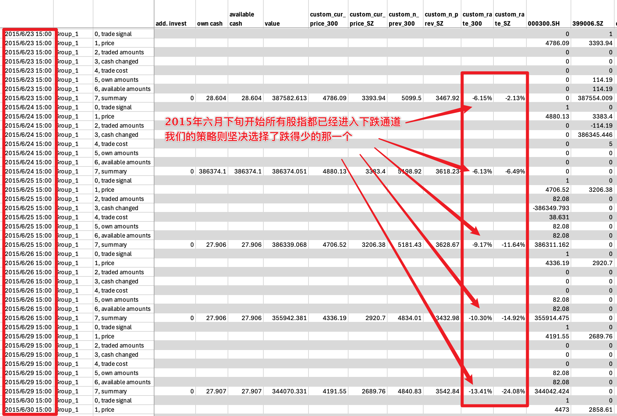
So in fact, at this time our strategy still chose the correct index. It’s just that because both indices were falling, our strategy held the one that fell less, reducing our losses.
But it was precisely our operations during this period that caused the biggest drawdown event in our ten-year investment history: from June 2025 all the way through to 2020, we were deeply trapped for as long as five years!!
Interpreting the Trading Report
Although the trading log contains all information in exhaustive detail, sometimes we don’t need to look at that much data. In that case, we can use the trading report.
The trading report is a compact version of the trading log file. It ignores all strategy run records without substantive trades and retains only all substantive trade records, including trade date, buy/sell direction, number of shares, price, total amount, transaction fee rate, and so on. Because it records only trades that actually occurred, the information is more compact:
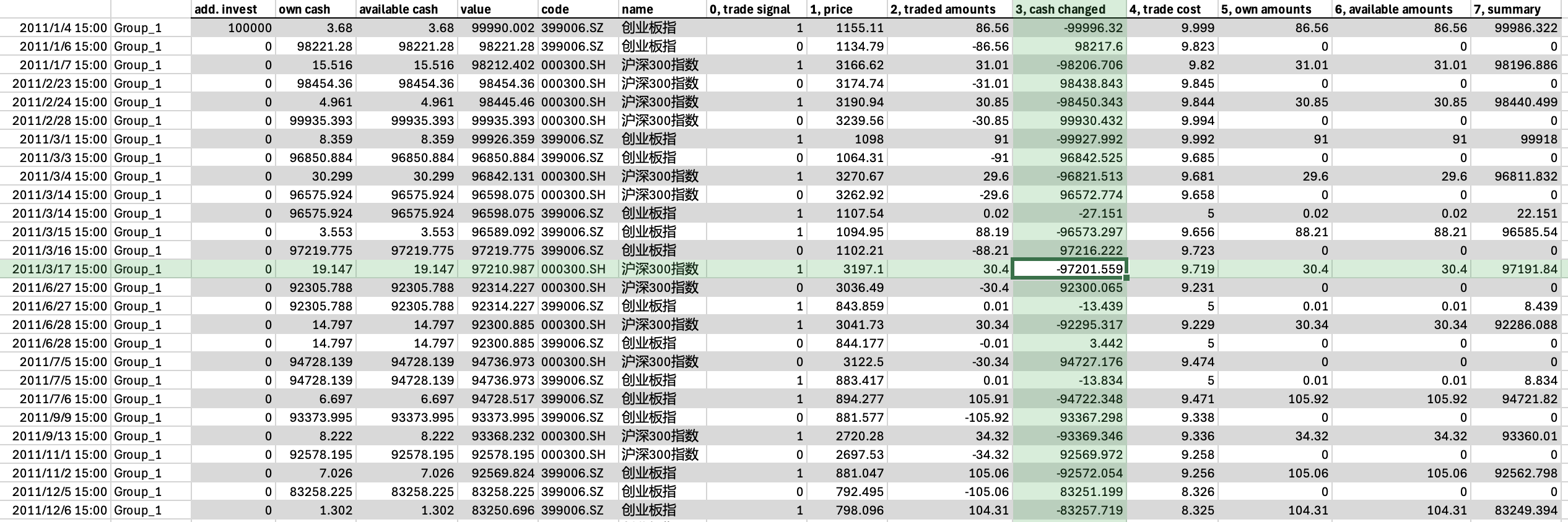
As you can see from the figure above, each row of the trading report records one actual trade record. If multiple trade records occur on the same day, they will be recorded on different rows.
Each row of the trading report records information such as the trading signal, trade price, trade quantity, cash change, transaction fee rate, and post-trade position size; the column names contain exactly the same information as the trading log.
7.6. Ideas for Improving the Strategy
Based on the above analysis of the trading strategy, we found that although this strategy achieved relatively good investment results, it performed poorly in controlling drawdowns: because it did not avoid the stock market crash period, it ended up deeply trapped.
Then, can we improve our strategy from here? The idea is simple. We can add a rule:
Calculate the increase of the two indices in the past 20 days every day, that is, the increase of today’s price relative to the price 20 days ago
If both indices are less than 0 on the stock selection day, then we will be empty the next day, and we will not hold any index
Otherwise, choose the index with the larger increase, hold it the next day, and sell the index with the smaller increase
We need to add a “filter condition” to the original simple stock selection rule to exclude the situation where both indices are less than 0. So, how to adjust in qteasy to reflect this new modification?
Improved strategy settings
qteasy’s built-in stock selection strategy provides a filter condition condition attribute. The default condition is condition='any', which means there is no filter condition. Now we need to filter out the return rate less than 0, so you can set condition='greater' and set the filter range ubound=0.
>>> op.set_parameter(0,
...                  condition='greater',  # 新增过滤条件:20日涨幅大于等于
...                  ubound=0.0,  # 过滤条件值:0
...                  )
Above settings are basically the same as the previous section, with two additional parameters:
condition='greater':it means a filter condition. The N-day increase must be greater than or equal to a certain value to participate in the stock selection. This value is set in theuboundparameter. That is, exclude stocks that are less than this value and make them unable to be selectedubound=0:Set to 0, so that only indices with an increase greater than or equal to 0 can be selected. Of course, it can also be set to other floating-point numbers
Improved results
Execute qt.run() directly according to the previous configuration. Here are the results:
>>> res=qt.run(op, visual=True, trade_log=True)
The output is as follows:
====================================
|                                  |
|         BACKTEST REPORT          |
|                                  |
====================================
qteasy running mode: 1 - History back testing
time consumption for operate signal creation: 146.7 ms
time consumption for operation back testing:  8.7 ms
investment starts on      2011-01-04 15:00:00
ends on                   2020-12-30 15:00:00
Total looped periods:     10.0 years.
-------------operation summary:------------
Only non-empty shares are displayed, call
"loop_result["oper_count"]" for complete operation summary
          Sell Cnt Buy Cnt Total Long pct Short pct Empty pct
000300.SH   113       99    212   26.7%     -0.0%     73.3%
399006.SZ    97      103    200   42.2%     -0.0%     57.8%

Total operation fee:     ¥   14,906.10
total investment amount: ¥  100,000.00
final value:              ¥  906,783.37
Total return:                   806.78%
Avg Yearly return:               24.68%
Skewness:                         -0.23
Kurtosis:                          4.86
Benchmark return:                60.32%
Benchmark Yearly return:          4.84%

------strategy loop_results indicators------
alpha:                            0.297
Beta:                             0.619
Sharp ratio:                      1.030
Info ratio:                       0.054
250 day volatility:               0.213
Max drawdown:                    28.88%
    peak / valley:        2018-01-24 / 2019-01-23
    recovered on:         2019-07-01


==================END OF REPORT===================
The visualization chart is as follows: 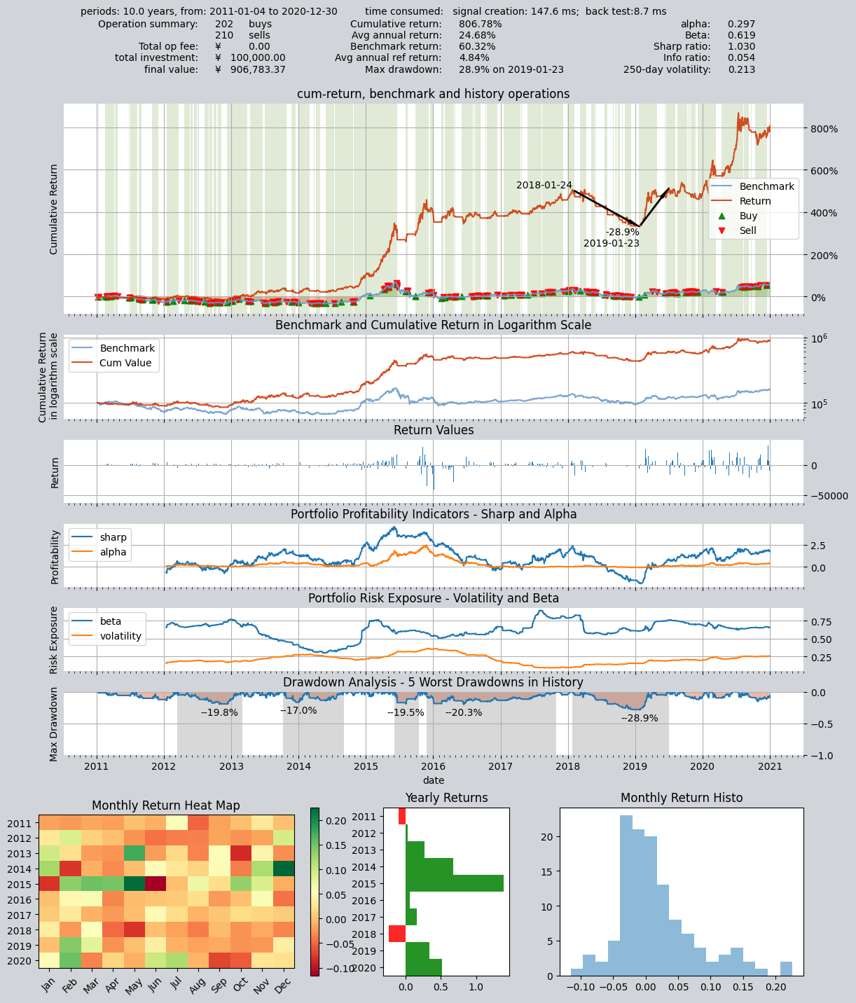
From the asset return chart, you can see that what used to be a solid block of green (fully invested throughout) has become alternating white and green (white intervals indicate being out of the market and holding cash). The drawdown has been greatly optimized: reduced from the original 50% drawdown to around 20%. And the total return has also increased significantly:
Total assets increased from a little over 500,000 before the improvement to a little over 900,000.
The total return increased from 300% to 806%.
The annualized return increased from 17% to 24.68%.
The maximum drawdown decreased from 50% to 28%.
By checking the transaction records, it is indeed that the strategy kept empty positions during the stock disaster at the end of June 2015, avoiding the one-way decline market.
7.7. Recap
In this tutorial, we familiarized ourselves with the trading strategy of qteasy through the creation, backtesting, and modification of a small-cap rotation trading strategy. We learned how to create a single strategy trader object by referencing the built-in trading strategy and run the strategy to obtain backtest results. Starting from the next tutorial, we will further discuss the built-in trading strategies of qteasy in detail and introduce the implementation of combination strategies. We will add more strategies to the trader object and set the combination method to achieve more complex effects through strategy combination, and understand more strategy control and types.