4. Multi-factor Stock Selection
Reference source: docs/_joinquant_migration_source/Example_04_Multifactor Stock Selection.ipynb First Markdown cell.
This strategy is triggered monthly, performing regression analysis on each stock using the Fama-French three-factor model to obtain its alpha value. Assuming the Fama-French three-factor model can fully explain the market, a negative alpha indicates that the market undervalues the stock, thus warranting a buy.
Strategy and Approach:
The market return, book-to-market ratio, and market capitalization of individual stocks were calculated, and the latter two were categorized. Based on the categorized portfolios, their market capitalization-weighted return, SMB, and HML were calculated. Regression was performed on each stock (assuming a risk-free rate of return of 0) to obtain the alpha value.
The 10 stocks with the lowest alpha values (less than 0) are selected for inclusion in the target pool. Stocks not in the target pool are removed, and the remaining stocks in the target pool are purchased with equal weighting.
Backtesting data: SHSE.000300 constituent stocks
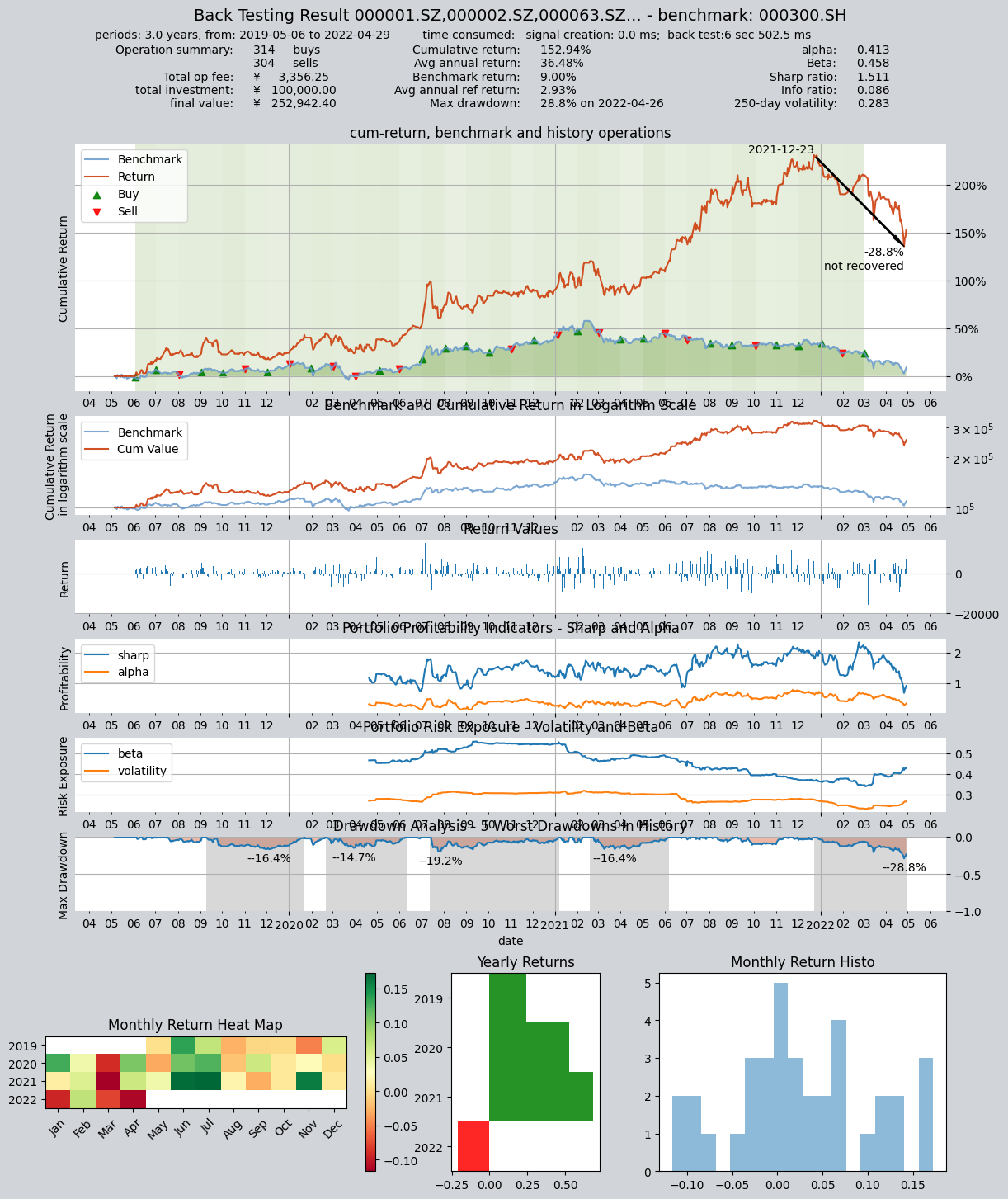
The backtesting period was from May 1, 2019 to May 1, 2022.
4.1. Define strategy
import qteasy as qt
import numpy as np
from qteasy import Parameter, StgData
def market_value_weighted(stock_return, mv, mv_cat, bp_cat, mv_target, bp_target):
    """ 根据mv_target和bp_target计算市值加权收益率

    """
    sel = (mv_cat == mv_target) & (bp_cat == bp_target)
    mv_total = np.nansum(mv[sel])
    mv_weight = mv / mv_total
    return_total = np.nansum(stock_return[sel] * mv_weight[sel])
    return return_total


class MultiFactors(qt.FactorSorter):

    def __init__(self, pars: tuple = (0.5, 0.3, 0.7)):
        super().__init__(
                name='MultiFactor',
                description='根据Fama-French三因子回归模型估算HS300成分股的alpha值选股',
                pars=[Parameter((0.01, 0.99), par_type='float', name='size_gate', value=0.5),  # 参数1:大小市值分类界限
                      Parameter((0.01, 0.49), par_type='float', name='pb_s', value=0.3),  # 参数2:小/中bp分界线
                      Parameter((0.50, 0.99), par_type='float', name='pb_l', value=0.7)],  # 参数3,中/大bp分界线
                data_types=[StgData('pb', freq='d', asset_type='E', window_length=20, use_latest_data_cycle=True),
                            StgData('total_mv', freq='d', asset_type='E', window_length=2, use_latest_data_cycle=True),
                            StgData('close', freq='d', asset_type='E', window_length=20, use_latest_data_cycle=True),
                            StgData('close-000300.SH', freq='d', asset_type='IDX', window_length=20, use_latest_data_cycle=True)],  # 执行选股需要用到的股票数据
                max_sel_count=10,  # 最多选出10支股票
                sort_ascending=True,  # 选择因子最小的股票
                condition='less',  # 仅选择因子小于某个值的股票
                lbound=0,  # 仅选择因子小于0的股票
                ubound=0,  # 仅选择因子小于0的股票
        )

    def realize(self):

        size_gate_percentile, bp_small_percentile, bp_large_percentile = self.get_pars('size_gate', 'pb_s', 'pb_l')
        # 读取投资组合的数据PB和total_MV的最新值
        pb, mv, closes, market_closes = self.get_data('pb_E_d', 'total_mv_E_d', 'close_E_d', 'close-000300.SH_IDX_d')
        pb = pb[-1]  # 当前所有股票的PB值
        mv = mv[-1]  # 当前所有股票的市值
        pre_close = closes[-2]  # 当前所有股票的前收盘价
        close = closes[-1]  # 当前所有股票的最新收盘价

        # 读取参考数据(r)
        market_pre_close = market_closes[-2]  # HS300的昨收价
        market_close = market_closes[-1]  # HS300的收盘价

        # 计算账面市值比,为pb的倒数
        bp = pb ** -1
        # 计算市值的50%的分位点,用于后面的分类
        size_gate = np.nanquantile(mv, size_gate_percentile)
        # 计算账面市值比的30%和70%分位点,用于后面的分类
        bm_30_gate = np.nanquantile(bp, bp_small_percentile)
        bm_70_gate = np.nanquantile(bp, bp_large_percentile)
        # 计算每只股票的当日收益率
        stock_return = pre_close / close - 1

        # 根据每只股票的账面市值比和市值,给它们分配bp分类和mv分类
        # 市值小于size_gate的cat为1,否则为2
        mv_cat = np.ones_like(mv)
        mv_cat += (mv > size_gate).astype('float')
        # bp小于30%的cat为1,30%~70%之间为2,大于70%为3
        bp_cat = np.ones_like(bp)
        bp_cat += (bp > bm_30_gate).astype('float')
        bp_cat += (bp > bm_70_gate).astype('float')

        # 获取小市值组合的市值加权组合收益率
        smb_s = (market_value_weighted(stock_return, mv, mv_cat, bp_cat, 1, 1) +
                 market_value_weighted(stock_return, mv, mv_cat, bp_cat, 1, 2) +
                 market_value_weighted(stock_return, mv, mv_cat, bp_cat, 1, 3)) / 3
        # 获取大市值组合的市值加权组合收益率
        smb_b = (market_value_weighted(stock_return, mv, mv_cat, bp_cat, 2, 1) +
                 market_value_weighted(stock_return, mv, mv_cat, bp_cat, 2, 2) +
                 market_value_weighted(stock_return, mv, mv_cat, bp_cat, 2, 3)) / 3
        smb = smb_s - smb_b
        # 获取大账面市值比组合的市值加权组合收益率
        hml_b = (market_value_weighted(stock_return, mv, mv_cat, bp_cat, 1, 3) +
                 market_value_weighted(stock_return, mv, mv_cat, bp_cat, 2, 3)) / 2
        # 获取小账面市值比组合的市值加权组合收益率
        hml_s = (market_value_weighted(stock_return, mv, mv_cat, bp_cat, 1, 1) +
                 market_value_weighted(stock_return, mv, mv_cat, bp_cat, 2, 1)) / 2
        hml = hml_b - hml_s

        # 计算市场收益率
        market_return = market_pre_close / market_close - 1

        coff_pool = []
        # 对每只股票进行回归获取其alpha值
        for rtn in stock_return:
            x = np.array([[market_return, smb, hml, 1.0]])
            y = np.array([[rtn]])
            # OLS估计系数
            coff = np.linalg.lstsq(x, y)[0][3][0]
            coff_pool.append(coff)

        # 以alpha值为股票组合的选股因子执行选股
        factors = np.array(coff_pool)

        return factors
4.2. Operational strategy
Set backtesting parameters and run the strategy.
shares = qt.filter_stock_codes(index='000300.SH', date='20190501')

alpha = MultiFactors()
op = qt.Operator(alpha, signal_type='PT', run_freq='ME')
qt.run(op=op,
       mode=1,
       invest_start='20160405',
       invest_end='20210201',
       asset_type='E',
       asset_pool=shares,
       trade_batch_size=100,
       sell_batch_size=1,
       trade_log=True,
      )
The results are as follows:
         ====================================
         |                                  |
         |       BACK TESTING RESULT        |
         |                                  |
         ====================================

    qteasy running mode: 1 - History back testing
    time consumption for operate signal creation: 0.0 ms
    time consumption for operation back looping:  6 sec 502.5 ms

    investment starts on      2019-05-06 00:00:00
    ends on                   2022-04-29 00:00:00
    Total looped periods:     3.0 years.

    -------------operation summary:------------
    Only non-empty shares are displayed, call
    "loop_result["oper_count"]" for complete operation summary

              Sell Cnt Buy Cnt Total Long pct Short pct Empty pct
    000063.SZ    1        1      2     2.7%      0.0%     97.3%
    000100.SZ    2        2      4     5.9%      0.0%     94.1%
    000157.SZ    3        3      6     8.6%      0.0%     91.4%
    000333.SZ    1        1      2     2.7%      0.0%     97.3%
    000338.SZ    2        2      4     5.5%      0.0%     94.5%
    000413.SZ    1        1      2     2.9%      0.0%     97.1%
    000423.SZ    1        1      2     2.7%      0.0%     97.3%
    000425.SZ    1        1      2     2.7%      0.0%     97.3%
    000625.SZ    2        2      4     5.6%      0.0%     94.4%
    000651.SZ    1        1      2     2.7%      0.0%     97.3%
    ...            ...     ...   ...      ...       ...       ...
    603185.SH    1        1      2     5.8%      0.0%     94.2%
    603290.SH    1        1      2     5.8%      0.0%     94.2%
    688005.SH    3        3      6     7.9%      0.0%     92.1%
    002756.SZ    1        1      2     2.7%      0.0%     97.3%
    600039.SH    1        1      2     2.8%      0.0%     97.2%
    600803.SH    1        1      2     2.9%      0.0%     97.1%
    688187.SH    1        1      2     2.9%      0.0%     97.1%
    000983.SZ    1        1      2     2.9%      0.0%     97.1%
    600732.SH    3        3      6     8.2%      0.0%     91.8%
    601699.SH    1        2      3     8.5%      0.0%     91.5%

    Total operation fee:     ¥    3,356.25
    total investment amount: ¥  100,000.00
    final value:              ¥  252,942.40
    Total return:                   152.94%
    Avg Yearly return:               36.48%
    Skewness:                         -0.19
    Kurtosis:                          3.08
    Benchmark return:                 9.00%
    Benchmark Yearly return:          2.93%

    ------strategy loop_results indicators------
    alpha:                            0.413
    Beta:                             0.458
    Sharp ratio:                      1.511
    Info ratio:                       0.086
    250 day volatility:               0.283
    Max drawdown:                    28.83%
        peak / valley:        2021-12-23 / 2022-04-26
        recovered on:         Not recovered!

    ===========END OF REPORT=============
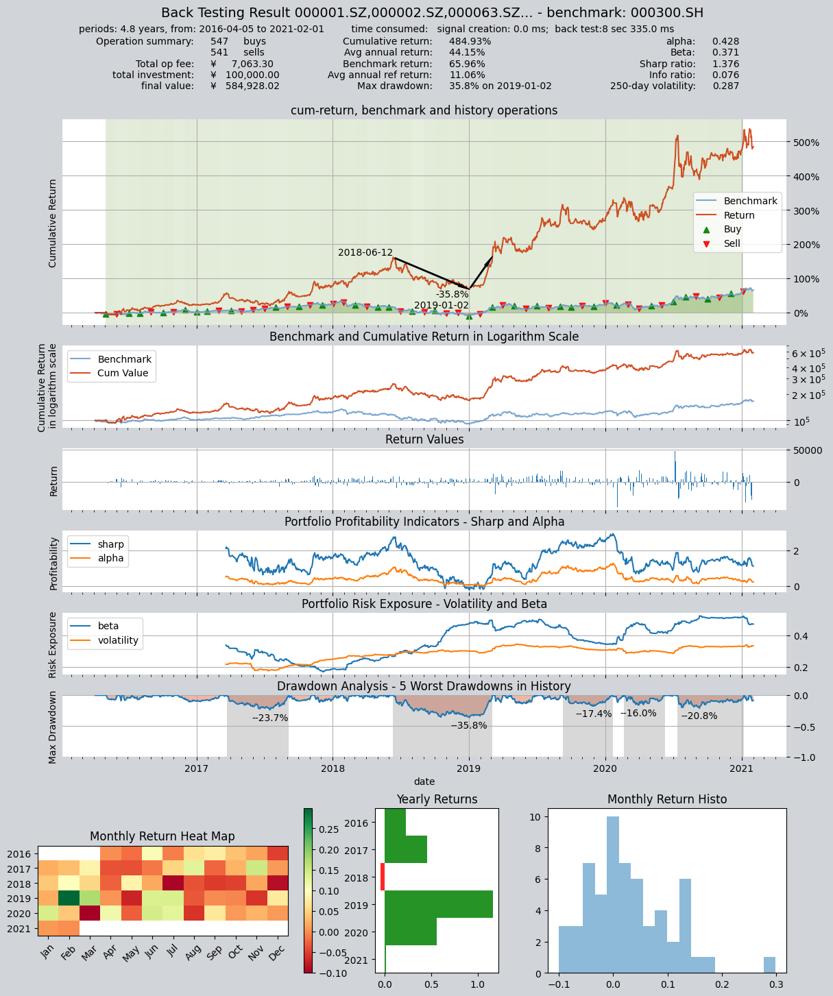
Set up another backtesting period from April 5, 2016 to February 1, 2021, and run the strategy. You can see that the strategy is effective in different periods.
shares = qt.filter_stock_codes(index='000300.SH', date='20190501')
alpha = MultiFactors()  # 实例化策略
op = qt.Operator(alpha, signal_type='PT')  # 创建Operator交易员对象,使用PT信号类型(仓位目标信号)
op.op_type = 'stepwise'
op.set_blender('1.0*s0')  # 设置仓位调整公式,仓位目标为1.0*s0,即持仓百分比总和等于100%
op.run(mode=1,
       invest_start='20160405',  # 回测起始时间
       invest_end='20210201',  # 回测结束时间
       asset_type='E',  # 股票
       asset_pool=shares,  # 股票池
       trade_batch_size=100,  # 交易最小批量
       sell_batch_size=1,  # 卖出最小批量
       trade_log=True,  # 产生交易记录
      )

print()
The results are as follows:
         ====================================
         |                                  |
         |       BACK TESTING RESULT        |
         |                                  |
         ====================================

    qteasy running mode: 1 - History back testing
    time consumption for operate signal creation: 0.0 ms
    time consumption for operation back looping:  8 sec 335.0 ms

    investment starts on      2016-04-05 00:00:00
    ends on                   2021-02-01 00:00:00
    Total looped periods:     4.8 years.

    -------------operation summary:------------
    Only non-empty shares are displayed, call
    "loop_result["oper_count"]" for complete operation summary

              Sell Cnt Buy Cnt Total Long pct Short pct Empty pct
    000063.SZ    2        2      4     3.4%      0.0%     96.6%
    000100.SZ    3        3      6     5.2%      0.0%     94.8%
    000157.SZ    1        1      2     1.8%      0.0%     98.2%
    000333.SZ    2        2      4     3.4%      0.0%     96.6%
    000338.SZ    1        1      2     1.7%      0.0%     98.3%
    000413.SZ    2        2      4     3.6%      0.0%     96.4%
    000596.SZ    1        1      2     1.8%      0.0%     98.2%
    000625.SZ    3        3      6     5.3%      0.0%     94.7%
    000629.SZ    1        1      2     1.7%      0.0%     98.3%
    000651.SZ    1        1      2     1.7%      0.0%     98.3%
    ...            ...     ...   ...      ...       ...       ...
    688005.SH    1        2      3     3.3%      0.0%     96.7%
    000733.SZ    1        1      2     1.8%      0.0%     98.2%
    002180.SZ    1        1      2     1.7%      0.0%     98.3%
    600039.SH    1        1      2     1.7%      0.0%     98.3%
    600803.SH    1        1      2     1.7%      0.0%     98.3%
    601615.SH    1        1      2     1.8%      0.0%     98.2%
    000983.SZ    2        2      4     3.3%      0.0%     96.7%
    600732.SH    3        4      7     6.7%      0.0%     93.3%
    600754.SH    1        1      2     1.8%      0.0%     98.2%
    601699.SH    1        1      2     1.7%      0.0%     98.3%

    Total operation fee:     ¥    7,063.30
    total investment amount: ¥  100,000.00
    final value:              ¥  584,928.02
    Total return:                   484.93%
    Avg Yearly return:               44.15%
    Skewness:                         -0.14
    Kurtosis:                          2.77
    Benchmark return:                65.96%
    Benchmark Yearly return:         11.06%

    ------strategy loop_results indicators------
    alpha:                            0.428
    Beta:                             0.371
    Sharp ratio:                      1.376
    Info ratio:                       0.076
    250 day volatility:               0.287
    Max drawdown:                    35.84%
        peak / valley:        2018-06-12 / 2019-01-02
        recovered on:         2019-03-05

    ===========END OF REPORT=============