8. Use built-in strategies
qteasy is a fully localized deployment and operation of quantitative trading analysis toolkit, with the following functions:
Access, clean, store, process, visualize, and use financial data
Create quantitative trading strategies and provide a large number of built-in basic trading strategies
Vectorized high-speed trading strategy backtesting and trading result evaluation
Optimization and evaluation of trading strategy parameters
Deployment and live operation of trading strategies
By this series of tutorials, you will fully understand the main functions and usage of qteasy through a series of practical examples.
8.1. Before you start
Before starting this tutorial, make sure you have mastered the following:
Install and configure
qteasy—— details please refer to QTEASY tutorial 1A local data source has been set up, and sufficient historical data has already been downloaded locally (including the trading calendar; basic information on stocks/funds/indices; price data for stocks/funds/indices; and financial indicators or other financial data—see QTEASY Tutorial 2 for details)
Learn to create a trader object, use a built-in trading strategy and backtest its historical performance, check the backtest log, understand how to adjust the running parameters or adjustable parameters of the strategy, and improve the performance of the strategy —— QTEASY tutorial 3
在QTEASY文档中,还能找到更多关于如何创建交易员对象运行策略,使用历史数据回测策略,检查回测交易记录,修改策略等等相关内容。对qteasy的基本使用方法还不熟悉的同学,可以移步那里查看更多详细说明。
8.2. Target of this chapter
In the previous tutorial section, we created an Operator trader object and had it run the first stock-picking trading strategy. However, in qteasy, a trader is capable of far more than just running a single trading strategy. In fact, the Operator object is like a real trader: it can simultaneously manage and run any number of trading strategies. These strategies can run separately at different times and frequencies, or many can run together in a batch; and strategies that run at the same time can also be “blended” in any specified way into the desired form.
You can think of a trader as a painter holding a palette with paints of different colors. They can use different colors to draw vivid lines, or mix several colors to create soft transitional tones. In this way, even if the painter has only a handful of paints, their brush can still blend millions of colors that make up the vast world.
This is exactly one of qteasy’s key design concepts: using the following two tools, the Operator trader object can combine and configure very simple trading strategies into very complex trading strategies, thereby enabling complex functionality. These two tools include:
Strategy Group: Traders can run multiple strategies in groups. Each group of trading strategies shares the same execution frequency (e.g., daily, hourly, or every minute) and the same execution timing (e.g., at the daily close or at 10:30 every day), allowing flexible control over when strategies run.
Blender Strategy Mixer: Trading strategies that run simultaneously within the same group will necessarily run at the same time. Each strategy will generate a set of trading signals according to its own logic, but this set of signals must be “merged” into a single set in some way. This merging is performed by the mixer
blender, which is specifically responsible for combining the trading signals generated by multiple strategies into one set. The merging logic is entirely determined by the user-definedblender stringcomposition string, giving the user full control.
In this chapter, we will learn how to use more built-in strategies in qteasy, how to make a trader run multiple trading strategies at the same time, and how to use the strategy mixer blender to generate different combination strategies using trading strategies.
At present, qteasy supports more than 70 built-in trading strategies, all of which are ready to use. For a complete list of built-in trading strategies, please refer to reference documents:
You can use the API below to get a list of all built-in trading strategies provided in qteasy:
import qteasy as qt
qt.built_ins()
The API above will return all built-in trading strategies in qteasy:
{'crossline': qteasy.built_in.CROSSLINE,
 'macd': qteasy.built_in.MACD,
 'dma': qteasy.built_in.DMA,
 'trix': qteasy.built_in.TRIX,
 'cdl': qteasy.built_in.CDL,
 'bband': qteasy.built_in.BBand,
 's-bband': qteasy.built_in.SoftBBand,
 'sarext': qteasy.built_in.SAREXT,
 'ssma': qteasy.built_in.SCRSSMA,
 'sdema': qteasy.built_in.SCRSDEMA,
 'sema': qteasy.built_in.SCRSEMA,
 'sht': qteasy.built_in.SCRSHT,
 'skama': qteasy.built_in.SCRSKAMA,
 'smama': qteasy.built_in.SCRSMAMA,
 ...}
The following list lists some of the built-in trading strategies that are ready to use in qteasy. For a complete list, please refer to reference documents
ID |
Name |
Description |
|---|---|---|
|
|
crossline timing strategy class, using the cross of long and short moving averages to determine the long and short states |
|
|
MACD timing strategy class, using the MACD moving average strategy to generate the target position percentage: |
|
|
DMA timing strategy |
|
|
TRIX timing strategy, using the triple-smoothed exponential moving average price of the stock price for long and short judgment: |
|
|
CDL timing strategy, find the cdldoji pattern that meets the requirements in the K-line chart |
|
|
Bollinger Band trading strategy, determine long and short positions based on the relationship between stock prices and Bollinger Band upper and lower bands, and generate trading signals when prices cross above or below the Bollinger Band lines. The moving average type of the Bollinger Band line cannot be selected |
|
|
Bollinger Band progressive trading strategy, determine long and short positions based on the relationship between stock prices and Bollinger Band upper and lower bands, and trading signals are not generated all at once, but gradually buy and sell. Calculate BBAND, check whether the price exceeds the upper or lower band of BBAND: |
|
|
Extended Parabolic SAR strategy, buy signal is issued when the index is greater than 0, and sell signal is issued when the index is less than 0 |
|
|
Single moving average cross strategy —— SMA moving average (simple moving average): set the position ratio according to the relative position of the stock price and the SMA moving average |
|
|
Single moving average cross strategy —— DEMA moving average (double exponential smoothing moving average): set the position ratio according to the relative position of the stock price and the DEMA moving average |
|
|
Single moving average cross strategy —— EMA moving average (exponential smoothing moving average): set the position ratio according to the relative position of the stock price and the EMA moving average |
… |
… |
Complete list of built-in strategies, please refer to reference documents |
Each built-in trading strategy has its own ID (e.g., crossline, macd, dma, etc. in the table above). Users can use this ID to obtain an instance of a built-in trading strategy and add it to a trader object for use. For example:
stg = qt.get_built_in_strategy('dma')
stg.info()
Output obtained:
================================ Strategy: DMA =================================
Strategy RULE-ITER(DMA)
Parameters: ['slow', 'long', 'diff'] = (12, 26, 9)
Date Types: close_ANY_d x 270
----------------------------- Iteration Properties -----------------------------
Allow multi pars        True
Multi-parameter not set
If you need to view a detailed explanation of each built-in trading strategy, such as the meaning of strategy parameters, signal generation rules, you can view the doc-string of each trading strategy:
For example:
qt.built_in_doc('Crossline', print_out=True)
You can see
Init signature: qt.built_in.TimingCrossline(pars:tuple=(35, 120, 0.02))
Docstring:
crossline择时策略类,利用长短均线的交叉确定多空状态

策略参数:
    s: int, 短均线计算日期;
    l: int, 长均线计算日期;
    m: float, 均线边界宽度(百分比);
信号类型:
    PT型:目标仓位百分比
信号规则:
    1,当短均线位于长均线上方,且距离大于l*m%时,设置仓位目标为1
    2,当短均线位于长均线下方,且距离大于l*mM时,设置仓位目标为-1
    3,当长短均线之间的距离不大于l*m%时,设置仓位目标为0

策略属性缺省值:
默认参数:(35, 120, 0.02)
数据类型:close 收盘价,单数据输入
采样频率:天
窗口长度:270
参数范围:[(10, 250), (10, 250), (0, 1)]
策略不支持参考数据,不支持交易数据
File:           ~/Library/CloudStorage/OneDrive-Personal/Projects/PycharmProjects/qteasy/qteasy/built_in.py
Type:           type
Subclasses:
In interactive python environments such as ipython, you can also use ? to display detailed information about built-in trading strategies, for example:
>>> qt.built_in.SelectingNDayRateChange?
You can see:
Init signature: qt.built_in.SelectingNDayRateChange(pars=(14,))
Docstring:
基础选股策略:根据股票以前n天的股价变动比例作为选股因子

策略参数:
    n: int, 股票历史数据的选择期
信号类型:
    PT型:百分比持仓比例信号
信号规则:
    在每个选股周期使用以前n天的股价变动比例作为选股因子进行选股
    通过以下策略属性控制选股方法:
    *max_sel_count:     float,  选股限额,表示最多选出的股票的数量,默认值:0.5,表示选中50%的股票
    *condition:         str ,   确定股票的筛选条件,默认值'any'
                                'any'        :默认值,选择所有可用股票
                                'greater'    :筛选出因子大于ubound的股票
                                'less'       :筛选出因子小于lbound的股票
                                'between'    :筛选出因子介于lbound与ubound之间的股票
                                'not_between':筛选出因子不在lbound与ubound之间的股票
    *lbound:            float,  执行条件筛选时的指标下界, 默认值np.-inf
    *ubound:            float,  执行条件筛选时的指标上界, 默认值np.inf
    *sort_ascending:    bool,   排序方法,默认值: False,
                                True: 优先选择因子最小的股票,
                                False, 优先选择因子最大的股票
    *weighting:         str ,   确定如何分配选中股票的权重
                                默认值: 'even'
                                'even'       :所有被选中的股票都获得同样的权重
                                'linear'     :权重根据因子排序线性分配
                                'distance'   :股票的权重与他们的指标与最低之间的差值(距离)成比例
                                'proportion' :权重与股票的因子分值成正比

策略属性缺省值:
默认参数:(14,)
数据类型:close 收盘价,单数据输入
采样频率:月
窗口长度:150
参数范围:[(2, 150)]
策略不支持参考数据,不支持交易数据
File:           ~/Library/CloudStorage/OneDrive-Personal/Projects/PycharmProjects/qteasy/qteasy/built_in.py
Type:           type
Subclasses:
8.3. Combination of multiple strategies
In qteasy, an Operator trader object can run any number of trading strategies in groups at the same time. When running, each of these strategies separately retrieves the historical data it needs and independently generates different trading signals. These signals are then combined into a set of trading signals and executed in a unified manner.
Users can use this feature to run multiple trading strategies with different focuses in a trader object at the same time. For example, one trading strategy monitors the stock price of individual stocks and generates selection signals based on the stock price, the second trading strategy is specifically responsible for monitoring the trend of the broader market, and determines the overall position based on the trend of the broader market. The third trading strategy is specifically responsible for stop loss and stop profit, and stops loss at specific times. The final trading signal is mainly based on the first trading strategy, but is restrained by the second strategy, and will be completely controlled by the third strategy when necessary.
Or, users can easily formulate a “committee” strategy, in which multiple strategies independently make trading decisions in a comprehensive strategy, and the final trading signal is determined by the “committee” vote composed of all sub-strategies. The voting method can be simple majority, absolute majority, weighted voting results, etc.
In the combined trading strategies above, each individual trading strategy is very simple and easy to define, yet combining them can produce a greater effect. At the same time, each sub-strategy is independent and can be freely combined into complex, comprehensive trading strategies. This avoids repeatedly developing strategies from scratch: you only need to rearrange and recombine the sub-strategies and redefine how they are combined to quickly build a series of complex, comprehensive trading strategies. This can greatly improve the efficiency of building trading strategies and shorten the cycle. Time is money.
Mixing trading signals refers to performing various operations or functions on trading signals. This can range from simple logical operations and addition/subtraction to complex custom functions. Any function that can be applied to an ndarray can be used to mix trading signals, as long as the final output trading signal is meaningful.
Define strategy combination method blender
In an Operator trader object, all trading strategies must be assigned to a strategy group. If there is more than one strategy in a group, a blender must be defined. If no blender is explicitly defined and the number of strategies exceeds 1, qteasy will create a default blender when running the Operator. However, for multi-strategy setups to run correctly, users need to define the blender themselves.
blender_str is a user-defined combination expression. Users use this expression to determine how different trading strategies are combined. This combination expression uses arithmetic operators, logical operators, functions, and other symbols to specify how strategy signals are combined. The blender expression can include the following elements:
The symbols supported in the blender expression are as follows:
Element |
Example |
Description |
|---|---|---|
Strategy number |
|
A string that starts with s and ends with a number. The number is the index of the strategy in |
Numbers |
|
Any legal number, the number involved in the expression operation |
Operators |
|
Numerical operators including |
Logical operators |
|
Logical operators such as |
Functions |
|
Supported functions can be seen in the table below |
Parentheses |
|
Group operation |
Example of blender
If there are three trading strategies in an Operator object (with serial numbers s0/s1/s2), the blender defined in the following ways is legal and available, and use Operator.set_blender() to set the blender:
Blender expression defined using arithmetic operators
's0 + s1 + s2'
In this case the trading signals generated by the three trading strategies will be added up to become the final trading signal. If the result of strategy 0 is buy 10%, the result of strategy 1 is buy 10%, and the result of strategy 2 is buy 30%, then the final result is buy 50%
Blender expression defined using logical operators:
's0 and s1 and s2'
In this case the final trading signal will only be formed when trading strategies 1, 2, and 3 all generate trading signals. For example, if the result of strategy 1 is buy, the result of strategy 2 is buy, and strategy 3 has no trading signal, then the final result is no trading signal.
Blender expressions can also include parentheses and some functions:
'max(s0, s1) + s2'
Meaning the sum of the maximum value of the results of strategies 1 and 2 and the result of strategy 3 becomes the final trading signal. If the result of strategy 1 is buy 10%, the result of strategy 2 is buy 20%, and the result of strategy 3 is buy 30%, the final result is buy 50%
A strategy can appear more than once in the blender expression, and pure numbers are also supported:
'(0.5 * s0 + 1.0 * s1 + 1.5 * s2) / 3 * min(s0, s1, s2)'
Above blender expression means: first calculate the weighted average of the three strategy signals (weights are 0.5, 1.0, 1.5 respectively), and then multiply by the minimum value of the three signals
Function parameters in the blender expression are defined in the function name:
'clip_-0.5_0.5(s0 + s1 + s2) + pos_2_0.2(s0, s1, s2)'
Above blender expression defines two different function operations, and the final result is obtained by adding the results. The first function is range clipping, after adding the three sets of strategy signals, the signal values less than -0.5 and greater than 0.5 are clipped, and the calculation result is obtained; the second function is position judgment function, which counts the time periods in the three sets of signals with a position greater than 0.2, defines them as “long positions”, and then counts the number of long position recommendations in the three strategies in each time period. If more than two strategies hold long position recommendations, the full position long position is output, otherwise the empty position is output.
Following functions are supported in the blender expression:
Functions |
Example of expression |
Description |
|---|---|---|
|
|
Absolute value function |
|
|
Average value function |
|
|
Average cumulative function |
|
|
Ceiing function |
|
|
Clip function |
|
|
Combo value function |
|
|
Committee function (equivalent to the cumulative position function pos)) |
|
|
exp function |
|
|
Floor function |
|
|
Logarithm function |
|
|
10-based logarithm function |
|
|
Maximum value function |
|
|
Minimum value function |
|
|
Accumulated position function |
|
|
Accumulated position function |
|
|
Power function |
|
|
Power function |
|
|
Square root function |
|
|
Strength cumulative function |
|
|
Strength cumulative function |
|
|
Combo value function |
|
|
Uniform function |
|
|
Vote function (equivalent to cumulative position function) |
Following methods can be used to set or get the blender of the strategy
operator.set_blender(blender_str=None, group_id=None)
To set the blender, pass in an expression blender_str directly. This expression will be automatically parsed and used to combine trading strategies. When using set_blender(), you can use the group_id parameter to specify which strategy group this blender is for. If group_id is not specified, this blender is used for all strategy groups by default.
operator.view_blender()
View the blender. Note that, for readability, the strategy codes s0, s1, and s2 in the blender expression will be automatically replaced with the specific strategy IDs, as shown in the example below:
>>> op = qt.Operator('dma, macd, trix')
>>> op.set_blender('(0.5 * s0 + 1.0 * s1 + 1.5 * s2) / 3 * min(s0, s1, s2)', group_id='Group_1')
>>> op.view_blender()
operator.view_blender() outputs a dictionary where the keys are strategy group IDs and the values are blender expressions. In the blender expression, s0, s1, and s2 have already been replaced with the specific strategy IDs:
The output is as follows:
{'Group_1': '(0.5 * dma + 1.0 * macd + 1.5 * trix) / 3 * min(dma, macd, trix)'}
If you specify the group_id parameter when calling view_blender(), it will only output the blender expression for that strategy group:
>>> op.view_blender(group_id='Group_1')
The output is as follows:
'(0.5 * dma + 1.0 * macd+ 1.5 * trix) / 3 * min(dma, macd, trix)'
Above example s0,s1,s2 are replaced by dma, macd, trix, but if the Operator contains multiple identical strategies, they will be automatically assigned different strategy IDs to distinguish:
>>> op = qt.Operator('dma, dma, dma')
>>> op.set_blender('(0.5 * s0 + 1.0 * s1 + 1.5 * s2) / 3 * min(s0, s1, s2)')
>>> op.view_blender('Group_1')
The output is as follows:
'(0.5 * dma_0 + 1.0 * dma_1 + 1.5 * dma_2) / 3 * min(dma_0, dma_1, dma_2)'
Example of using blender
An example is used below to demonstrate how blender works:
We generate a trader object and run five DMA trading strategies at the same time, but the five trading strategies have different adjustable parameters. At this time, we can understand that the trader runs five of the same trading logic at the same time, but these five trading logics are configured with different parameters, so under the same input conditions, different trading signals are generated, which means that the five trading strategies have their own emphasis, some are good at capturing long-term variables, and some are good at tracking short-term trends.
Now, the same five trading strategies, but we will use three different examples to show three different blending methods, to show you that even if the same trading strategy and trading parameters, in the same historical interval, different blending methods can also affect the final trading results.
First blending method: Weighted average blending
The first blending method takes a weighted average of the results of the five trading strategies. The weights for each trading strategy are as follows:
s0: weight 0.8
s1: weight 1.2
s2: weight 2.0
s3: weight 0.5
s4: weight 1.5
To achieve the weighted-average blending above, we can define the following blender expression. It means: first multiply the results of the five trading strategies by their respective weights, then divide by the sum of the weights (i.e., 5) to obtain the weighted-average result:
(0.8*s0+1.2*s1+2*s2+0.5*s3+1.5*s4)/5
Next, we set this blender expression on the trader object, run the strategies, and obtain the backtest results:
# 创建一个交易员对象,同时运行五个相同的dma交易策略,这些交易策略运行方式相同,但是设置不同的参数后,会产生不同的交易信号。我们通过不同的策略组合方式,得到不同的回测结果
op = qt.Operator('dma, dma, dma, dma, dma')
# 分别给五个不同的交易策略设置不同的策略参数,使他们产生不同的交易信号
op.set_parameter(stg_id=0, par_values=(132, 200, 24))
op.set_parameter(stg_id=1, par_values=(124, 187, 51))
op.set_parameter(stg_id=2, par_values=(103, 81, 16))
op.set_parameter(stg_id=3, par_values=(48, 111, 148))
op.set_parameter(stg_id=4, par_values=(104, 127, 58))

op.set_blender('(0.8*s0+1.2*s1+2*s2+0.5*s3+1.5*s4)/5')

# 运行策略
res = qt.run(op, mode=1, invest_start='20160405', invest_end='20210201')
The resulting backtest report is as follows: annualized return 5.51%, Sharpe ratio 0.44. For how to interpret the backtest report, please refer to the relevant content in Tutorial Section 3.
Here we are not focusing on how to improve the performance of the trading strategies. Instead, we focus on how the same trading strategies produce different backtest results under different blending methods, and these differences in backtest results come entirely from the different blending methods.
====================================
|                                  |
|         BACKTEST REPORT          |
|                                  |
====================================
qteasy running mode: 1 - History back testing
time consumption for operate signal creation: 171.1 ms
time consumption for operation back testing:  3.2 ms
investment starts on      2016-04-05 15:00:00
ends on                   2021-01-29 15:00:00
Total looped periods:     4.8 years.
-------------operation summary:------------
Only non-empty shares are displayed, call
"loop_result["oper_count"]" for complete operation summary
          Sell Cnt Buy Cnt Total Long pct Short pct Empty pct
000300.SH   370      354    724   88.1%     -0.0%     11.9%

Total operation fee:     ¥    3,847.81
total investment amount: ¥  100,000.00
final value:              ¥  129,535.45
Total return:                    29.54%
Avg Yearly return:                5.51%
Skewness:                         -0.90
Kurtosis:                         12.22
Benchmark return:                63.94%
Benchmark Yearly return:         10.80%

------strategy loop_results indicators------
alpha:                           -0.060
Beta:                             1.311
Sharp ratio:                      0.440
Info ratio:                      -0.041
250 day volatility:               0.125
Max drawdown:                    18.49%
    peak / valley:        2018-01-26 / 2019-01-03
    recovered on:         2019-03-05


==================END OF REPORT===================
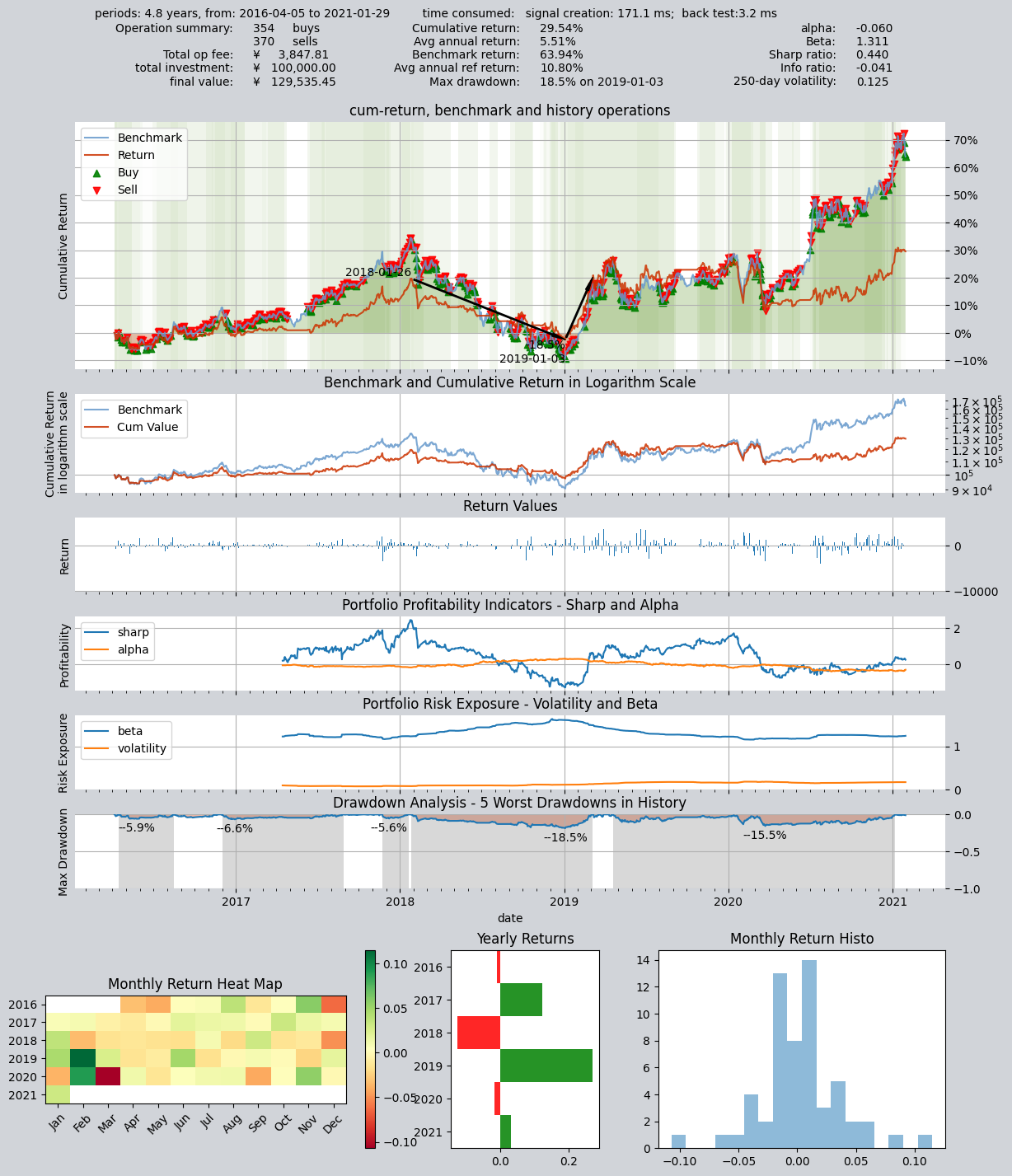
Examine profit curve chart above carefully, and you will notice that the background of the chart is drawn with different shades of green stripes. These stripes represent the position ratio in that period of time. White represents an empty position, that is, not holding any stocks at all, and the darkest green represents 100% holding stocks. The green in the middle represents the position ratio between 0 and 100%, and the higher the position ratio, the darker the color of the stripes.
Because the outputs of the five trading strategies are combined as a weighted average, any change in the output of any one strategy will cause the final trading signal to change. This also makes the number of trades over the entire backtest period very frequent (a total of 370 sell operations and 354 buy operations), and the position ratio also fluctuates frequently between 0% and 100%.
You can see from the chart that there are different shades of green in the entire trading history interval. If you examine each holding interval very carefully, you will find that the holding ratio of these intervals corresponds exactly to the blending results of the five trading strategies at that time: when all trading strategies “decide unanimously” to buy full position, the weighted average result is 100% buy, but as long as one or more strategies decide to hold an empty position, the final weighted average result is to hold a certain percentage of stocks, which is equal to the weighted average result of the five strategy signals. The final result is that the position ratio fluctuates between 0% and 100%, and the time of completely empty position and completely full position is not long.
That also means that we cannot completely avoid one-way decline market by empty position, but always maintaining a certain position can better grasp the upward channel.
Meanwhile, you should also be able to observe that because the position is flexibly adjusted, the position (the depth of green) in the one-way decline market is obviously lower, and the position in the rising market is higher, which is exactly what we expect.
Next, let’s take a look at a completely different blending method:
Second blending method: Committee voting
This blender lets the same five trading strategies form a “committee” to determine the position through equal voting, and the position must be one of the two results of “non-black or white”: either full position or empty position. The expression is as follows:
At this point we need to use the special function supported by blender_str, the “committee function”, cmt_N_T(s0, s1, ...). This function means: when the number of strategies that simultaneously generate a non-flat signal (with absolute signal value > T) is greater than N, output fully invested long (1) or fully invested short (-1); otherwise output flat (0). Therefore, when N=3 and T=0, the expression is as follows:
cmt_3_0(s0, s1, s2, s3, s4)
This is equivalent to creating a committee consisting of five trading strategies: only when at least three strategies simultaneously recommend a fully invested long position will the committee output a fully invested long recommendation; otherwise it outputs a flat (no position) recommendation.
So the final result is that the position ratio is either 100% (when three or more strategies output a fully invested recommendation) or 0% (when fewer than three strategies output a fully invested recommendation). In a one-way down market, the position ratio is either 100% or 0%, with no intermediate state. The trader Operator is essentially executing a trading strategy that determines the position based on the vote of a five-member investment committee. Each committee member has their own view (because their parameters differ), but the final decision is determined by the majority.
op.set_blender('cmt_3_0(s0, s1, s2, s3, s4)')  # 将委员会混合函数设置为blender表达式
# 运行策略
res = qt.run(op, mode=1)
The results are as follows: annualized return 6.43, Sharpe ratio 0.487
====================================
|                                  |
|         BACKTEST REPORT          |
|                                  |
====================================
qteasy running mode: 1 - History back testing
time consumption for operate signal creation: 179.3 ms
time consumption for operation back testing:  3.2 ms
investment starts on      2016-04-05 15:00:00
ends on                   2021-01-29 15:00:00
Total looped periods:     4.8 years.
-------------operation summary:------------
Only non-empty shares are displayed, call
"loop_result["oper_count"]" for complete operation summary
          Sell Cnt Buy Cnt Total Long pct Short pct Empty pct
000300.SH    10       9      19   57.2%     -0.0%     42.8%

Total operation fee:     ¥      452.82
total investment amount: ¥  100,000.00
final value:              ¥  135,022.14
Total return:                    35.02%
Avg Yearly return:                6.43%
Skewness:                         -0.74
Kurtosis:                         11.60
Benchmark return:                63.94%
Benchmark Yearly return:         10.80%

------strategy loop_results indicators------
alpha:                           -0.034
Beta:                             1.001
Sharp ratio:                      0.487
Info ratio:                      -0.026
250 day volatility:               0.138
Max drawdown:                    22.60%
    peak / valley:        2019-04-19 / 2020-07-24
    recovered on:         Not recovered!


==================END OF REPORT===================
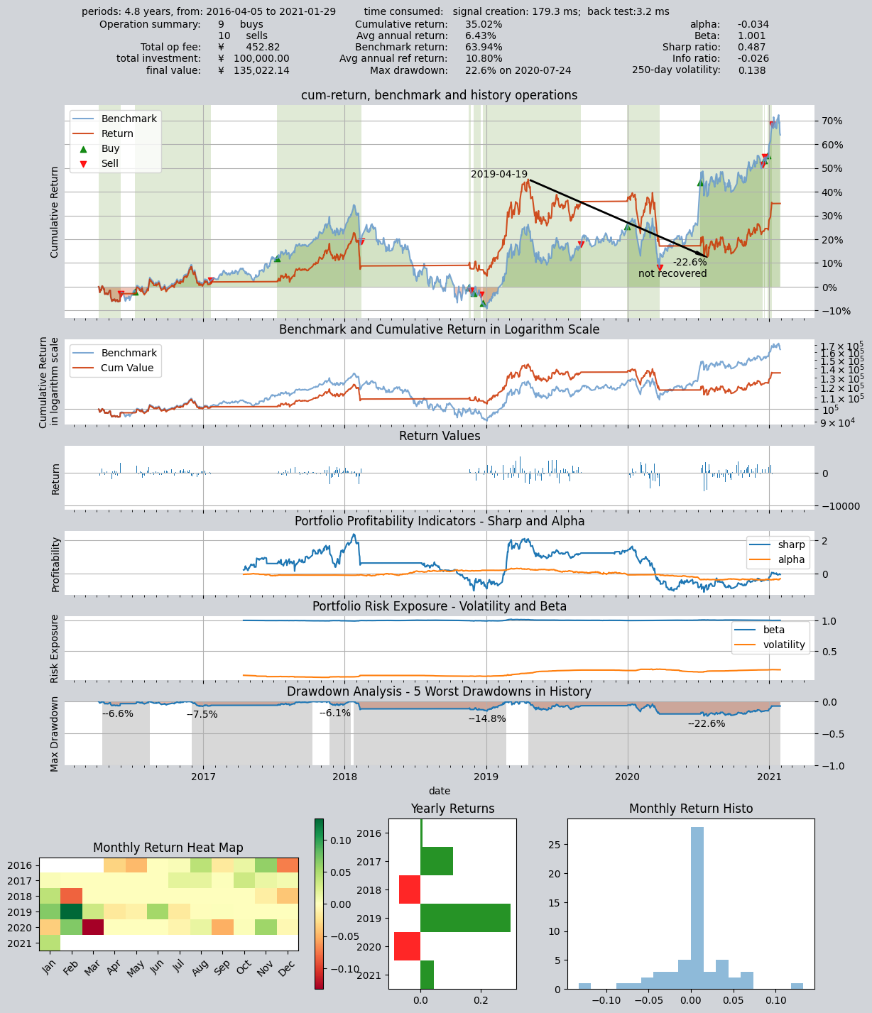
You must have noticed that this time the output is very different from the previous one: in the last backtest the position ratio changed gradually (the shade of the green bands in the background of the return chart represents the position ratio), whereas this time it’s black-or-white—either fully invested or flat—and the number of trades is also greatly reduced, with only nine buys and ten sells in total. If you analyze the trade log carefully, you’ll find that it goes fully invested only when three trading strategies vote in favor of being fully invested; the rest of the time it stays flat. Therefore, in a one-way down market, the equity curve is a straight line. But when fully invested, if the stock falls, there is no way to reduce losses by appropriately trimming the position.
Next, we still use this committee, but now as long as two votes are cast for full position, the final position will be full position:
Third blending method: Committee voting
The third portfolio construction method: still a committee strategy, but the voting threshold for outputting a fully invested long position is changed to 2 votes, i.e., as long as two strategies think it should output long, it will do so.
op.set_blender('pos_2_0(s0, s1, s2, s3, s4)')
# 运行策略
res = qt.run(op, mode=1)
The results are as follows: annualized return 8.46%, Sharpe ratio 0.612
====================================
|                                  |
|         BACKTEST REPORT          |
|                                  |
====================================
qteasy running mode: 1 - History back testing
time consumption for operate signal creation: 180.0 ms
time consumption for operation back testing:  3.5 ms
investment starts on      2016-04-05 15:00:00
ends on                   2021-01-29 15:00:00
Total looped periods:     4.8 years.
-------------operation summary:------------
Only non-empty shares are displayed, call
"loop_result["oper_count"]" for complete operation summary
          Sell Cnt Buy Cnt Total Long pct Short pct Empty pct
000300.SH    12       10     22   71.5%     -0.0%     28.5%

Total operation fee:     ¥      548.27
total investment amount: ¥  100,000.00
final value:              ¥  147,914.95
Total return:                    47.91%
Avg Yearly return:                8.46%
Skewness:                         -0.64
Kurtosis:                          8.61
Benchmark return:                63.94%
Benchmark Yearly return:         10.80%

------strategy loop_results indicators------
alpha:                           -0.018
Beta:                             1.001
Sharp ratio:                      0.612
Info ratio:                      -0.018
250 day volatility:               0.154
Max drawdown:                    22.34%
    peak / valley:        2019-04-19 / 2020-07-24
    recovered on:         Not recovered!


==================END OF REPORT===================
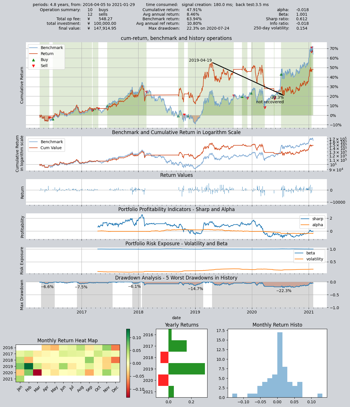
Compare the second chart and the third chart, you will find that the full position interval has obviously become longer, this is because the strategy that used to require three votes to be fully positioned, now only needs two votes, so it is easier to achieve full position
8.4. Recap
Alright—by now you should have a preliminary understanding of how trading strategies can be blended. Our tutorial will continue: qteasy offers even more ways to implement the trading strategies you want. In fact, although the core of qteasy is designed as a vectorized strategy engine that is conducive to high-speed backtesting and high-speed execution, it still takes sufficient flexibility into account. In theory, you can implement any type of trading strategy you can imagine.
Meanwhile, qteasy’s backtesting framework has also made quite a lot of special designs, which can completely avoid you inadvertently importing “future functions” into the trading strategy, ensuring that your trading strategy is completely based on past data during backtesting. At the same time, many preprocessing techniques and JIT techniques are used to compile the kernel key functions to achieve a running speed no less than that of C language.
However, in order to achieve theoretically infinite possible trading strategies, it may not be enough to use only built-in trading strategies and strategy blending. Some specific trading strategies, or some particularly complex trading strategies cannot be created by built-in strategy blending. This requires us to use the Strategy base class provided by qteasy to create a custom trading strategy based on certain rules.
In the next section of the qteasy tutorial, we will use an example to introduce how to create a custom trading strategy, how to define the basic parameters of the strategy, how to define the data types required by the strategy, how to set the logic for generating trading signals…