Back Test and evaluate Strategy

qteasy all trading strategies are implemented through the qteast.Operator (trader) object for backtesting and operation. The Operator object is a strategy container, and a trader can simultaneously manage multiple different trading strategies, even if these trading strategies have different operating timings and frequencies, or different purposes. For example, one strategy is used for stock selection, another strategy is used for market timing, and another strategy is used for risk control. Users can flexibly add or modify the strategies in the Operator object.

After handing over the strategy to Operator, as long as the asset class for trading, the size of the asset pool, and the operating timing and frequency of each strategy are set, the Operator object will start the corresponding trading strategy at the appropriate time, generate strategy signals, and mix (blend) all strategy signals to resolve them into trading signals.

For more information about the Operator object, please refer to the qteasy documentation.

qteasy provides two ways to create trading strategies:

Using built-in trading strategy combinations
- qteasy provides a variety of built-in trading strategies for users to use without manual creation. By referencing the name of the built-in strategy (for detailed documentation on all built-in strategies), users can quickly establish strategies and also mix multiple simple strategies into more complex composite strategies.
Through the strategy class to create strategies
- If the user’s strategy is very complex, a strategy can be customized through the qteasy.Strategy class.

Creating trading strategies, backtesting the trading results of trading strategies using historical data, and evaluating the trading results are one of the core functions of qteasy. qteasy summarizes a series of trading strategies through a trader object (Operator), and simulates the operation of trading strategies within a set historical time period using the qt.run() function, generating trading signals, simulating trading using historical prices, generating trading results, calculating evaluation indicators, and outputting them in visual form as charts.

Here is an example of a common fund timing investment strategy, demonstrating the following content:

Create a simple DMA timing investment strategy, create a trader object using this strategy, and demonstrate how to modify and add strategies
With qt.configure() set the relevant environment variables, use the historical data of the CSI 300 index for the past 10 years to backtest the strategy performance
Optimize the strategy parameters using the historical data of the CSI 300 index for the past 10 years, and finally demonstrate the results after optimization

First we import the qteasy module. To print charts online, use matplotlib inline to set the chart printing mode to online printing.

Create Strategy and Operator objects

Every trading strategy in qteasy is defined as a trading strategy (Strategy) object. Each trading object contains a series of trading rules, which include three aspects:

Strategy running rules include the frequency of strategy operation, the type of historical data used, and the length of the historical data window, which define how the strategy operates and how to use historical data
Signal generation rules The rules for generating trading signals, that is, how to generate what kind of trading signals based on relevant historical data, which is the core of the trading strategy
Trading signal types The different types of trading signals determine how the simulation trading module processes trading signals

In qteasy, trading strategies are executed by the trader object (Operator). At the same time, only one Operator object can run, but the same trader can execute one or more trading strategies simultaneously. These trading strategies can trade on the same portfolio, and users can define specific “mixing” methods to combine multiple simple trading strategies into a complex trading strategy.

Create Strategy object

Createing a Strategy object is easiest using the qt.built_in module, and it can also be created when creating the Operator object.

import qteasy as qt
# 通过qt内置策略模块创建一个DMA则时策略
stg = qt.built_in.DMA()
# 通过stg.info()可以查看策略的主要信息：
stg.info()

Strategy_type:      RuleIterator
Strategy name:      DMA
Description:        Quick DMA strategy, determine long/short position according to differences of moving average prices with simple timing strategy
Strategy Parameter: (12, 26, 9)

Strategy Properties     Property Value
-------------------------------------------------
Param. count            3
Param. types            ['int', 'int', 'int']
Param. range            [(10, 250), (10, 250), (5, 250)]
Run parameters          d @ close
Data types              ['close']
Data parameters         270 d

We can see the basic information of this trading strategy from the output. In addition to the name and description, important information includes:

Strategy Parameter. The strategy parameter is the external parameter required during the operation of the strategy. Depending on the different strategy rules, the parameters used by the strategy are also different. These parameters affect the operation of the strategy, and different parameters affect the output of the strategy. For example, in a dual moving average strategy, the calculation period of the long moving average and the calculation period of the short moving average are two strategy parameters.
Parameter Types / Range: Different strategy parameters can greatly affect the final result of a strategy. After setting the value range and type of parameters, qteasy can search for the best parameters in the parameter space through different methods to optimize the performance of the strategy.
Strategy Data Frequency / Sample Frequency. The frequency of strategy operation and the frequency of data required, such as once a week, once a month, or once a minute, etc. Generally speaking, the data frequency is related to the execution frequency.
Data Types: The historical data types required to run the strategy. For the DMA strategy, only the closing price is needed.

If you want to see all built-in strategies, you can use the qt.built_ins() function. If you do not give the function parameters, it will display a list of all built-in strategies. If you give parameters, it will display detailed information about the specified built-in strategy. For example:

qt.built_ins('dma')

Result:

 DMA择时策略

    策略参数：
        s, int, 短均线周期
        l, int, 长均线周期
        d, int, DMA周期
    信号类型：
        PS型：百分比买卖交易信号
    信号规则：
        在下面情况下产生买入信号：
        1， DMA在AMA上方时，多头区间，即DMA线自下而上穿越AMA线后，输出为1
        2， DMA在AMA下方时，空头区间，即DMA线自上而下穿越AMA线后，输出为0
        3， DMA与股价发生背离时的交叉信号，可信度较高

    策略属性缺省值：
    默认参数：(12, 26, 9)
    数据类型：close 收盘价，单数据输入
    采样频率：天
    窗口长度：270
    参数范围：[(10, 250), (10, 250), (8, 250)]
    策略不支持参考数据，不支持交易数据

More built-in strategy functions include:

`qt.built_ins(stg_id=None)`

If stg_id=None, display a list of all built-in strategies, otherwise display detailed information about the specified built-in strategy.

`qt.built_in_list(stg_id=None)`

If stg_id=None, return a list of all built-in strategies, otherwise return detailed information about the specified built-in strategy.

`qt.built_in_strategies(stg_id=None)`

If stg_id=None, return a list of all built-in strategies, otherwise return detailed information about the specified built-in strategy.

`qt.get_built_in_strategy(stg_id)`

According to the given built-in strategy ID, return the built-in strategy object.

Create Operator object

Creating an Operator object can be done using qt.Operator(). After creating an Operator object, all trading strategies are run by the trader object. When creating the trader object, you can specify how to handle trading signals and how to run the trading:

`qt.Operator(strategies=None, signal_type=None, op_type=None)`

strategies: The trading strategies in the trader object can be one or more trading strategies, or a list of a trading strategy. If no trading strategy is specified, an empty trader object is created, and the trading strategy can be added or deleted later. Once a trading strategy is added, the trader object assigns a unique ID to each trading strategy, which can be used to reference this trading strategy. At the same time, the trader object will automatically assign an operating timing to each trading strategy according to the operating frequency and timing of the strategy. Only when the operating timing arrives will the trader object execute this trading strategy and generate trading signals.
signal_type: The type of trading signal can be 'pt', 'ps', or 'vs', defaulting to 'pt', which represents target holding ratio signals, percentage trading signals, and quantity trading signals, respectively. Different types of trading signals determine how the trader object processes trading signals and how the trader object mixes the trading signals of multiple trading strategies into a single trading signal.
op_type: The operating mode of the trader object can be 'batch' or 'realtime', defaulting to 'batch', which represents batch operation mode and real-time operation mode, respectively. In batch operation mode, the trader object will generate trading signals in advance in backtesting or optimization mode, and then perform simulated trading in batches, which is faster. In real-time operation mode, the trader object will generate trading signals and immediately simulate trading. After generating simulated trading results, it will generate the next trading signal, which is suitable for real trading operation mode or special backtesting mode.

For qteasy, the trading signals of trading strategies and the trading orders of stocks/funds are two different concepts.

All trading strategies are based on historical data to generate trading signals, while the trader object generates trading orders based on trading signals, simulating the trader’s trading behavior, and ultimately generating trading results.

Three types of strategy signals

In qteasy, trading signals are floating-point numbers, and the same trading signal can represent different meanings, which are interpreted by the trader object as different trading orders. The meaning of the trading signal is determined by the signal type of the trader object, which can be 'pt', 'ps', or 'vs', representing target holding ratio signals, percentage trading signals, and quantity trading signals, respectively.

There are three types of trading signals:

PT: This trading signal represents the target holding ratio, which means that the value of the held stock accounts for the proportion of total assets. For example, when the current total assets are 1 million yuan, 0.2 means controlling the holding quantity of a certain stock or fund to make its market value 20% of 1 million yuan, which is 200,000 yuan. In this case, the number of stocks bought or sold depends on the current number of stocks held. If the current number of stocks held is 0, then buy 200,000 yuan worth of stocks. If the current value of stocks held is 300,000 yuan, then sell 100,000 yuan worth.
PS: This trading signal directly represents the buy/sell ratio. In this case, the number of stocks bought or sold is unrelated to the current number of stocks held, but only related to the total assets. If the total assets are 1 million yuan, 0.2 means buying 200,000 yuan worth of stocks.
VS: In this case, the trading signal directly represents the buy/sell quantity. In this case, the number of stocks bought or sold is unrelated to total assets or the number of shares held. 2000 means buying 2000 shares of stock.

Furthermore, if the generated trading orders differ based on the type of account operated by the trader (such as a stock account or futures account), the generated trading orders will also differ. The specific explanation is shown in the following table:

账户类型	信号类型	交易信号	信号含义	信号举例	交易订单举例
股票账户	PT	sig > 0	持有该资产，并使持有资产的市值为总资产的sig倍	0.5	根据当前持有的资产比例确定交易订单，如果已经满仓持有，则卖掉50%仓位，如果持仓为0，则买入至50%仓位
		sig = 0	清空全部持有的资产，持有资产为0	0	根据当前持有的资产比例确定交易订单，如果持仓则卖掉全部持仓，如果没有持仓则不交易
		sig < 0	无意义	N/A	N/A
	PS	sig > 0	买入该资产，买入的金额占总资产的比例为sig	0.5	总资产为100,000，则此时花费50,000元金额买入资产(含手续费)
		sig = 0	不进行任何操作	0	不进行任何操作
		sig < 0	卖出该资产，卖出的部分占当前持有数量的比例为sig	-0.5	假设当前持有1000股，则此时应卖出500股
	VS	sig > 0	买入该资产，买入的数量为sig	500	买入500股
		sig = 0	不进行任何操作	0	不进行任何操作
		sig < 0	卖出该资产，卖出的数量为abs(sig)	-500	卖出500股
期货账户 (未实现)	PT	sig > 0	平掉所有空仓，开多仓，并使持有合约价值为总资产的sig倍	1.5	假设总资产为100,000，开多仓持有总价150,000的合约 *当保证金比例<1时，持仓比例可以大于100%
		sig = 0	平掉全部持有的仓位，持有头寸为0	0	平掉所有持有的多仓和空仓
		sig < 0	平掉所有多仓，开空仓，并使持有合约价值为总资产的sig倍	-1.5	总资产为100,000，则开空仓持有总价150,000的合约 * 如果保证金比例<1时，持空仓比例可以大于100%
	PS	sig > 0	如果持有空仓：平部分空仓，平空仓的数量占总持有的比例为sig	0.5	如果总持仓为1,000手，则此时平仓500手 * 此时sig必须小于等于1
		sig > 0	如果持有多仓：开多仓，开仓的合约价值占总资产的比例为sig	1.5	如果总资产为100,000，则开多仓持有总价150,000元的合约 * 如果保证金比例<1时，sig可以大于1
		sig = 0	不进行任何操作	0	不进行任何操作
		sig < 0	如果持有多仓：平部分多仓，平仓的数量占总持有的比例为sig	0.5	如果总持仓为1,000手，则此时平仓500手 * 此时sig必须小于等于1
		sig < 0	如果持有空仓：开空仓，开仓的合约价值占总资产的比例为sig	1.5	如果总资产为100,000，则开空仓持有总价150,000元的合约 * 如果保证金比例<1时，sig可以大于1
	VS	sig > 0	平空仓或开多仓，开平仓的数量为sig。如果持有空头数量超过sig则忽略剩余部分	1500	如果持有1500手以上空头仓位，则平仓1500手，如果当前没有持仓，则开多仓持有1500手合约
		sig = 0	不进行任何操作	0	不进行任何操作
		sig < 0	平多仓或开空仓，开平仓的数量为sig。如果持有多头数量超过sig则忽略剩余部分	-500	如果持有1500手以上多头仓位，则平仓1500手，如果当前没有持仓，则开空仓持有1500手合约

Blending Trading Signals

Although the same Operator object can only generate one type of signal at the same time, since the Operator object can accommodate an infinite number of different trading strategies, it can also produce an infinite number of sets of the same type of trading strategies. To save computational overhead during trading backtesting, avoid conflicting or duplicate trading signals from occupying computing resources, and to increase the flexibility of trading signals, all trading signals should be mixed into a set before being sent to the backtesting program for testing.

However, in an Operator object, the trading signals generated by different strategies may run at different trading prices. For example, some strategies generate opening price trading signals, while others generate closing price trading strategies. In this case, different trading price signals should not be mixed. But other than that, as long as the trading prices are the same, all signals should be mixed.

Blending trading signals means various operations or functions of trading signals, from simple logical operations and addition/subtraction operations to complex custom functions. As long as they can be applied to an ndarray function, they can theoretically be used to mix trading signals, as long as the final output trading signal is meaningful.

Signal blending is based on a series of predefined operations and functions, which are referred to as “atomic functions” or “operators”. Users use these “operators” to manipulate the trading signals generated by the Operator object and transform multiple sets of trading signals into a unique set of trading signals while maintaining their shape and meaningful numbers.

Signals are blended by a blending expression blender, for example, s0 and (s1 + s2) * avg(s3, s4)

blender expressions support the following functions:

Element	Example	Description
Strategy index	`s1`	A string starting with s and ending with a number, where the number is the sequence number of the strategy in `Operator`, representing the trading signal generated by this strategy
Digits	`-1.35`	Any valid number, a number that participates in expression operations
Operators	`+`	Includes `'+-*/^'` and other four arithmetic operators
Logical Operators	`and`	Supports logical operators in forms like `'&\|~'` and `'and/or/not'`
Functions	`sum()`	Supported functions are shown in the table below
Perentheses	`()`	Combined Operations

Fore more examples of blending expressions, please refer to qteasy Tutorial 04 - Use built-in strategies

op = qt.Operator()

OPERATOR INFO:
=========================
Information of the Module
=========================
Total 0 operation strategies, requiring 0 types of historical data:

0 types of back test price types:
[]

Operator object is a strategy container, and any number of trading strategies can be added to an Operator object. At the same time, the blending method (blender), trading signal processing method, and trading operation method of the trading strategy can be managed in the Operator object.

Normal Operator attributes and methods are as follows:

Get basic information of Operator object

`op.info()`

Print important information of Operator object

`op.strategies`

Get the list of all trading strategies in the Operator object

`op.strategy_ids`

Get the IDs of all trading strategies in the Operator object

`op.strategy_count`

Get the number of trading strategies in the Operator object

`op.signal_type`

Signal type of Operator object, representing the meaning and processing method of trading signals:

‘pt’: Target holding ratio signal, in this mode, the trader focuses on the holding ratio of each component stock in a portfolio. By timely buying and selling, maintain the holding ratio of each component stock at a target value;
‘ps’: Percentage trading signal, in this mode, the trader focuses on the proportion of trading signals generated at regular intervals, buying or selling stocks according to the trading signals proportionally
‘vs’: Quantity trading signal, in this mode, the trader focuses on the trading signals generated at regular intervals, buying or selling a certain number of stocks according to the trading signals

`op.op_type`

Running mode of Operator object:

‘batch’: Batch operation mode, in backtesting or optimization mode, generate trading lists in advance, and then perform simulated trading in batches, which is faster
‘realtime’: Real-time operation mode, generate trading signals and immediately simulate trading. After generating simulated trading results, generate the next trading signal, which is suitable for real-time operation mode or special backtesting mode

Get Trading Strategy

`op.get_stg(stg_id)`

Get strategy object by strategy ID. The following methods have the same effect and can be used to get strategy by number sequence

stg = op.get_stg(stg_id)
stg = op[stg_id] 
stg = op[stg_idx]

Add or Modify Trading Strategy

`op.add_strategy(stg, **kwargs)`

Add a strategy to Operator, and set strategy parameters at the same time

`op.add_strategies(strategies)`

Add a series of strategies to Operator in batches, and cannot set strategy parameters at the same time

`op.remove_strategy(id_or_pos=None)`

Remove a strategy from Operator

`op.clear_strategies()`

Remove all trading strategies in Operator

Set Strategy Parameters or Operator Parameters

`op.set_parameter(stg_id, pars=None, opt_tag=None, par_range=None, par_types=None, data_freq=None, run_freq=None, window_length=None, data_types=None, strategy_run_timing=None, **kwargs)`

Given a trading strategy ID, set the strategy parameters or other attributes of this trading strategy

`op.set_blender(price_type=None, blender=None)`

Set the blending method of trading strategy. When there are multiple trading strategies in Operator, each trading strategy runs separately to generate multiple sets of trading signals, and then outputs a set of trading signals according to user-defined rules for trading

We can use the following code to add the newly created DMA strategy to Operator and set the necessary strategy parameters

All parameter settings can be done using the operator.set_parameter method, and multiple parameters can be passed in at the same time. By setting the strategy’s opt_tag, you can control whether the strategy participates in optimization, while the par_range parameter defines the parameter space needed for strategy optimization. At this time, we do not know what the optimal DMA timing parameters are for the past 15 years of the CSI 300 index, so we can input a few random parameters to conduct a backtest and see how it goes.

op.clear_strategies()
op.add_strategy(stg, pars=(26, 35, 189), opt_tag=1)
print(f'Operator strategies: {op.strategies}')
print(f'Strategy IDs are: {op.strategy_ids}')
op.info(verbose=True)

Operator strategies: [RULE-ITER(DMA)]
Strategy IDs are: ['custom']
OPERATOR INFO:
=========================
Information of the Module
=========================
Total 1 operation strategies, requiring 1 types of historical data:
close
1 types of back test price types:
['close']
for backtest histoty price type - close: 
[RULE-ITER(DMA)]:
no blender
Parameters of GeneralStg Strategies:
Strategy_type:      RuleIterator
Strategy name:      DMA
Description:        Quick DMA strategy, determine long/short position according to differences of moving average prices with simple timing strategy
Strategy Parameter: (26, 35, 189)

Strategy Properties     Property Value
---------------------------------------
Parameter count         3
Parameter types         ['int', 'int', 'int']
Parameter range         [(10, 250), (10, 250), (10, 250)]
Data frequency          d
Sample frequency        d
Window length           270
Data types              ['close']

=========================

Configure qteasy’s backtesting parameters

Backtesting can begin after the Operator object is created and strategies are added

qteasy provides rich environment parameters to control the specific process of backtesting. All environment parameter variable values can be viewed through qt.Configuration() and set through qt.Configure().

`qt.configuration()`

Check qteasy running environment variables

`qt.configure()`

Set qteasy running environment variables

Environment variable parameters related to backtesting include:

Target stocks/index for backtesting
Start and end time period of backtesting
Initial investment amount for backtesting
Trading fees and trading rules for backtesting
Benchmark index for evaluating trading results

All the above backtesting trading parameters can be set through qt.configure()

qt.configure(
    mode=1,  # 设置运行模式为：1-回测模式
    benchmark_asset = '000300.SH',  # 设置交易评价基准（类型由系统根据代码自动推断）
    asset_pool = '000300.SH',  # 设置交易资产组合
    asset_type = 'IDX',  # 交易资产组合的资产类型
    trade_batch_size = 0.01,  # 设置允许最小交易批量（最小0.01）
    invest_start = '20100105',  # 设置交易开始日期
    invest_end = '20201231',  # 设置交易终止日期
    invest_cash_amounts = [1000000],  # 设置初始交易投资金额为十万元
    visual=True  # 输出可视化交易结果图表
)

Start qteasy and run Operator

`qt.run(operator, **config)`

Start running Operator. Depending on the mode of operation, qteasy will enter different operating modes and output different results:

mode 0 Real-time mode: Read the most recent (real-time) data and generate the latest trading signals. In this mode, you can set qteasy to execute periodically, read the latest data periodically, and generate real-time trading signals periodically
mode 1 Backtesting mode: Read historical data over a period of time, generate trading signals using that data, and simulate trading to output the results of simulated trading
mode 2 Optimization mode: Read historical data over a period of time, repeatedly run the same set of trading strategies but use different parameter combinations to search for the best-performing strategy parameters during this period

Operator can be started by running qteasy.run(operator, **config), where **config is the test environment parameter. The environment variables passed in as parameters in qt.run() are only valid for this run, but the environment variables set in qt.configure() will remain valid until changed next time.

Final backtesting assets are 190,000 yuan, annualized return is only 4.83%, Sharpe ratio is only 0.0783, and return is lower than the CSI 300 index during the same period

qt.run(op)

The system will automatically read historical data, conduct backtesting, complete result evaluation, and print the backtesting report after running qteasy.

Backtesting report will include the following information:

Total time taken for backtesting
Backtesting interval start and end dates, duration, and other information
Trading statistics: such as number of buys, number of sells, full position ratio, empty position ratio, total trading costs, etc.
Return information: initial investment amount, final asset amount, total return rate, annualized return rate, benchmark total return rate, benchmark annualized return rate, kurtosis and skewness of return rate
Indicators for portfolio evaluation: Alpha, Beta, Sharpe ratio, information ratio, volatility, and maximum drawdown

         ====================================
         |                                  |
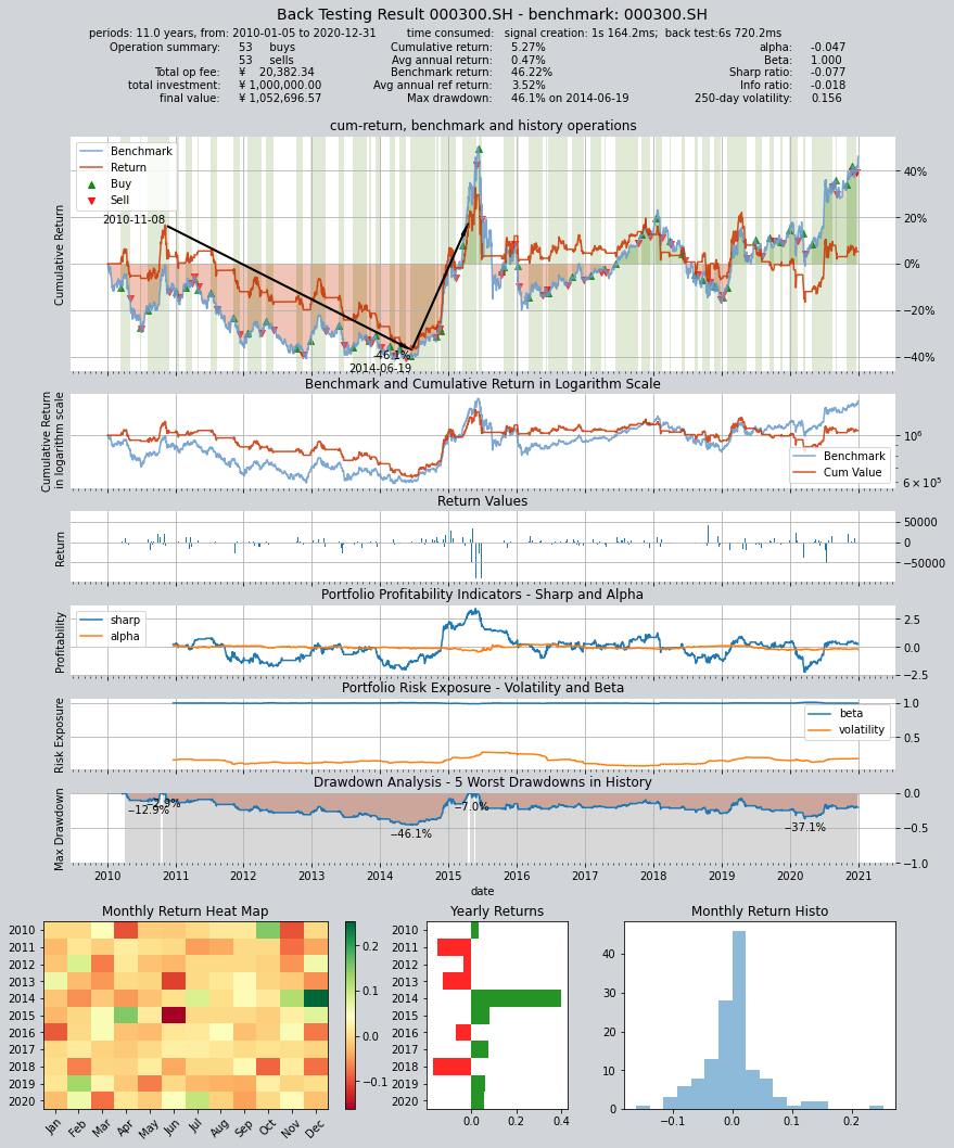
         |       BACK TESTING RESULT        |
         |                                  |
         ====================================
    
    qteasy running mode: 1 - History back testing
    time consumption for operate signal creation: 1s 164.2ms
    time consumption for operation back looping:  6s 720.2ms
    
    investment starts on      2010-01-05 00:00:00
    ends on                   2020-12-31 00:00:00
    Total looped periods:     11.0 years.
    
    -------------operation summary:------------
    
              Sell Cnt Buy Cnt Total Long pct Short pct Empty pct
    000300.SH    53       53    106   54.0%      0.0%     46.0%   
    
    Total operation fee:     ¥   20,382.34
    total investment amount: ¥1,000,000.00
    final value:              ¥1,052,696.57
    Total return:                     5.27% 
    Avg Yearly return:                0.47%
    Skewness:                         -0.76
    Kurtosis:                         11.44
    Benchmark return:                46.22% 
    Benchmark Yearly return:          3.52%
    
    ------strategy loop_results indicators------ 
    alpha:                           -0.047
    Beta:                             1.000
    Sharp ratio:                     -0.077
    Info ratio:                      -0.018
    250 day volatility:               0.156
    Max drawdown:                    46.12% 
        peak / valley:        2010-11-08 / 2014-06-19
        recovered on:         2015-04-17
     
    ===========END OF REPORT=============

Except for the backtesting report, a visual chart will also be printed, showing detailed information of the entire backtesting process.

Following information will be displayed in this information chart:

Return rate curve of the entire backtesting history (showing holding period, buy/sell points, benchmark return rate curve, and maximum drawdown period)
Return rate curve and benchmark in logarithmic scale
Daily return rate change chart
Rolling Sharpe ratio and alpha rate change chart (portfolio profitability evaluation)
Rooling volatility and beta rate change chart (portfolio risk evaluation)
Drawdown analysis chart (submarine chart)
Monthly and annual return rate heat map and bar chart
Montly return rate statistical frequency histogram

png

Large number of parameters can be set in the simulated trading process of qteasy, such as:

Total amount of funds invested, date, or set to invest in batches multiple times;
Trading fees for buying and selling, including commission rate, minimum fee, fixed fee, and slippage. Various rates can be set separately for buying and selling
Delivery time of buying and selling transactions, that is, T+N delivery system
Minimum batch size for buying and selling transactions, such as whether fractional shares are allowed, or whether integer shares or even hundreds of shares are required for trading

Final printed backtesting results are the final results after considering all the above trading parameters, so you can see the total trading costs. For detailed trading parameter settings, please refer to the detailed documentation.

Additionally, qteasy also provides several indicators about strategy performance: alpha and beta are 0.067 and 1.002 respectively, while the Sharpe ratio is 0.041. The maximum drawdown occurred from August 3, 2009 to July 10, 2014, with a drawdown of 35.0%, and it was not until December 16, 2014 that it turned around.

In the above backtesting results, we set the parameter visual=False. If we set visual=True, we can get visual backtesting results in the form of charts, and provide visual information:

Capital curve of investment strategy
Benchmark data (CSI 300 index) historical curve
Purchase and sell points (displayed with red and green arrows on the reference data)
Holding period (green indicates holding)
Investment strategy evaluation indicators (alpha, sharp, etc.)
Drawdown analysis (showing the five largest drawdowns)
Return rate heat map, mountain accumulation chart, and other charts

qteasy provides rich strategy backtesting options, such as:

Start and end date of backtesting
Investment strategy evaluation indicators
If negative positions are allowed during backtesting (used to simulate futures trading short-selling behavior, or special futures trading simulation algorithms can be used)

More options can be found in the detailed documentation

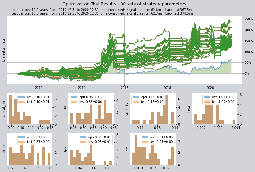
Optimization of single timing strategy

Obviously, the unoptimized parameters cannot achieve ideal backtesting results, so we need to perform an optimization

We can set the optimization method and control the optimization process by setting various parameters of the context object: The meanings of the following parameters are as follows:

Optimization method is set to 1, using Monte Carlo optimization, which has good optimization ability for larger parameter space
Output result quantity is set to 30
Number of iterations in the optimization process is 1000
If the parallel parameter is set to True, all cores of the multi-core processor will be used for parallel computing to save time

Then start the optimization, using the perfs_dma and pars_dma variables to store the optimization results. A progress bar will be displayed during the optimization process, and the optimization results will be displayed after completion

pars_dma = qt.run(op, 
                  mode=2,
                  opti_method=1,
                  opti_sample_count=1000,
                  opti_start='20101231',
                  opti_end='20201231',
                  opti_cash_dates='20101231',
                  test_start='20101231',
                  test_end='20201231',
                  test_cash_dates='20101231',
                  parallel=True)
print(f'optimization completed, 50 parameters found, they are\n'
      f'{pars_dma}')

[########################################]1000/1000-100.0%  best performance: 340613.629
Optimization completed, total time consumption: 38"247
[########################################]30/30-100.0%  best performance: 340613.629
==================================== 
|                                  |
|       OPTIMIZATION RESULT        |
|                                  |
====================================

qteasy running mode: 2 - Strategy Parameter Optimization

investment starts on 2010-12-31 00:00:00
ends on 2020-12-31 00:00:00
Total looped periods: 10.0 years.
total investment amount: ¥   100,000.00
Reference index type is 000300.SH at IDX
Total Benchmark rtn: 66.59% 
Average Yearly Benchmark rtn rate: 5.23%
statistical analysis of optimal strategy messages indicators: 
total return:        161.24% ± 29.73%
annual return:       10.01% ± 1.18%
alpha:               0.048 ± 0.014
Beta:                1.001 ± 0.001
Sharp ratio:         0.625 ± 0.089
Info ratio:          0.013 ± 0.004
250 day volatility:  0.151 ± 0.006
other messages indicators are listed in below table

    Strategy items  Sell-outs Buy-ins ttl-fee      FV      ROI   Benchmark rtn  MDD 
0    (147, 157, 57)    25.0     25.0  1,213.16 231,710.13 131.7%     66.6%     38.1%
1    (88, 108, 127)    16.0     15.0  1,009.93 233,554.10 133.6%     66.6%     44.3%
2    (105, 160, 29)    21.0     20.0  1,344.78 232,247.09 132.2%     66.6%     26.4%
3    (149, 194, 24)    19.0     19.0  1,062.61 233,932.11 133.9%     66.6%     33.4%
4    (105, 185, 25)    18.0     17.0  1,094.07 236,171.54 136.2%     66.6%     40.6%
5    (86, 147, 107)    11.0     10.0    668.08 234,827.39 134.8%     66.6%     39.7%
6    (88, 157, 101)    11.0     10.0    715.01 236,851.09 136.9%     66.6%     31.6%
7    (144, 181, 57)    19.0     19.0  1,093.20 240,445.16 140.4%     66.6%     33.8%
8     (94, 165, 78)    12.0     11.0    724.66 240,825.90 140.8%     66.6%     38.1%
9    (68, 113, 142)    13.0     12.0    819.42 244,805.70 144.8%     66.6%     42.5%
10     (80, 64, 57)    30.0     30.0  1,767.04 245,084.54 145.1%     66.6%     28.8%
11   (101, 124, 65)    23.0     22.0  1,726.89 245,504.45 145.5%     66.6%     30.7%
12   (150, 189, 33)    20.0     20.0  1,142.62 246,185.41 146.2%     66.6%     34.3%
13   (119, 200, 30)    12.0     11.0    705.66 248,111.42 148.1%     66.6%     24.1%
14   (52, 111, 136)    14.0     13.0    810.29 254,764.49 154.8%     66.6%     40.5%
15    (55, 151, 87)    14.0     13.0    896.37 248,370.33 148.4%     66.6%     38.2%
16    (98, 129, 45)    22.0     21.0  1,480.50 252,764.13 152.8%     66.6%     37.1%
17    (101, 59, 50)    27.0     26.0  1,505.08 255,487.88 155.5%     66.6%     28.8%
18   (179, 240, 25)    19.0     19.0  1,149.62 259,380.09 159.4%     66.6%     33.8%
19   (82, 127, 144)    12.0     11.0    810.46 268,321.59 168.3%     66.6%     37.4%
20   (44, 135, 117)    13.0     12.0    741.60 268,837.16 168.8%     66.6%     42.6%
21   (103, 127, 57)    22.0     21.0  1,628.33 269,776.04 169.8%     66.6%     30.3%
22   (128, 152, 92)    15.0     15.0    883.81 272,170.16 172.2%     66.6%     32.6%
23    (91, 198, 13)    17.0     16.0  1,209.55 277,214.25 177.2%     66.6%     43.3%
24  (102, 110, 129)    26.0     25.0  2,056.58 311,876.36 211.9%     66.6%     33.4%
25   (129, 204, 16)    14.0     14.0    840.49 279,142.60 179.1%     66.6%     32.6%
26    (90, 185, 45)    11.0     10.0    735.84 279,320.37 179.3%     66.6%     40.6%
27  (104, 111, 107)    30.0     29.0  2,207.23 317,371.14 217.4%     66.6%     41.0%
28   (101, 150, 24)    23.0     22.0  2,012.97 331,442.65 231.4%     66.6%     26.4%
29   (104, 142, 87)    15.0     14.0  1,044.25 340,613.63 240.6%     66.6%     23.5%

===========END OF REPORT=============

[########################################]30/30-100.0%  best performance: 340613.629
==================================== 
|                                  |
|       OPTIMIZATION RESULT        |
|                                  |
====================================

qteasy running mode: 2 - Strategy Parameter Optimization

investment starts on 2010-12-31 00:00:00
ends on 2020-12-31 00:00:00
Total looped periods: 10.0 years.
total investment amount: ¥   100,000.00
Reference index type is 000300.SH at IDX
Total Benchmark rtn: 66.59% 
Average Yearly Benchmark rtn rate: 5.23%
statistical analysis of optimal strategy messages indicators: 
total return:        161.24% ± 29.73%
annual return:       10.01% ± 1.18%
alpha:               0.048 ± 0.014
Beta:                1.001 ± 0.001
Sharp ratio:         0.625 ± 0.089
Info ratio:          0.013 ± 0.004
250 day volatility:  0.151 ± 0.006
other messages indicators are listed in below table

    Strategy items  Sell-outs Buy-ins ttl-fee      FV      ROI   Benchmark rtn  MDD 
0    (105, 160, 29)    21.0     20.0  1,344.78 232,247.09 132.2%     66.6%     26.4%
1    (88, 108, 127)    16.0     15.0  1,009.93 233,554.10 133.6%     66.6%     44.3%
2    (147, 157, 57)    25.0     25.0  1,213.16 231,710.13 131.7%     66.6%     38.1%
3    (105, 185, 25)    18.0     17.0  1,094.07 236,171.54 136.2%     66.6%     40.6%
4    (88, 157, 101)    11.0     10.0    715.01 236,851.09 136.9%     66.6%     31.6%
5    (149, 194, 24)    19.0     19.0  1,062.61 233,932.11 133.9%     66.6%     33.4%
6    (144, 181, 57)    19.0     19.0  1,093.20 240,445.16 140.4%     66.6%     33.8%
7    (86, 147, 107)    11.0     10.0    668.08 234,827.39 134.8%     66.6%     39.7%
8    (68, 113, 142)    13.0     12.0    819.42 244,805.70 144.8%     66.6%     42.5%
9     (94, 165, 78)    12.0     11.0    724.66 240,825.90 140.8%     66.6%     38.1%
10   (150, 189, 33)    20.0     20.0  1,142.62 246,185.41 146.2%     66.6%     34.3%
11   (101, 124, 65)    23.0     22.0  1,726.89 245,504.45 145.5%     66.6%     30.7%
12     (80, 64, 57)    30.0     30.0  1,767.04 245,084.54 145.1%     66.6%     28.8%
13   (119, 200, 30)    12.0     11.0    705.66 248,111.42 148.1%     66.6%     24.1%
14    (55, 151, 87)    14.0     13.0    896.37 248,370.33 148.4%     66.6%     38.2%
15    (98, 129, 45)    22.0     21.0  1,480.50 252,764.13 152.8%     66.6%     37.1%
16   (52, 111, 136)    14.0     13.0    810.29 254,764.49 154.8%     66.6%     40.5%
17    (101, 59, 50)    27.0     26.0  1,505.08 255,487.88 155.5%     66.6%     28.8%
18   (179, 240, 25)    19.0     19.0  1,149.62 259,380.09 159.4%     66.6%     33.8%
19   (82, 127, 144)    12.0     11.0    810.46 268,321.59 168.3%     66.6%     37.4%
20   (44, 135, 117)    13.0     12.0    741.60 268,837.16 168.8%     66.6%     42.6%
21   (103, 127, 57)    22.0     21.0  1,628.33 269,776.04 169.8%     66.6%     30.3%
22   (128, 152, 92)    15.0     15.0    883.81 272,170.16 172.2%     66.6%     32.6%
23    (91, 198, 13)    17.0     16.0  1,209.55 277,214.25 177.2%     66.6%     43.3%
24   (129, 204, 16)    14.0     14.0    840.49 279,142.60 179.1%     66.6%     32.6%
25    (90, 185, 45)    11.0     10.0    735.84 279,320.37 179.3%     66.6%     40.6%
26  (104, 111, 107)    30.0     29.0  2,207.23 317,371.14 217.4%     66.6%     41.0%
27  (102, 110, 129)    26.0     25.0  2,056.58 311,876.36 211.9%     66.6%     33.4%
28   (101, 150, 24)    23.0     22.0  2,012.97 331,442.65 231.4%     66.6%     26.4%
29   (104, 142, 87)    15.0     14.0  1,044.25 340,613.63 240.6%     66.6%     23.5%

===========END OF REPORT=============

png

optimization completed, 50 parameters found, they are
[(147, 157, 57), (105, 160, 29), (88, 108, 127), (149, 194, 24), (86, 147, 107), (105, 185, 25), (88, 157, 101), (144, 181, 57), (94, 165, 78), (68, 113, 142), (80, 64, 57), (101, 124, 65), (150, 189, 33), (119, 200, 30), (55, 151, 87), (98, 129, 45), (52, 111, 136), (101, 59, 50), (179, 240, 25), (82, 127, 144), (44, 135, 117), (103, 127, 57), (128, 152, 92), (91, 198, 13), (129, 204, 16), (90, 185, 45), (102, 110, 129), (104, 111, 107), (101, 150, 24), (104, 142, 87)]

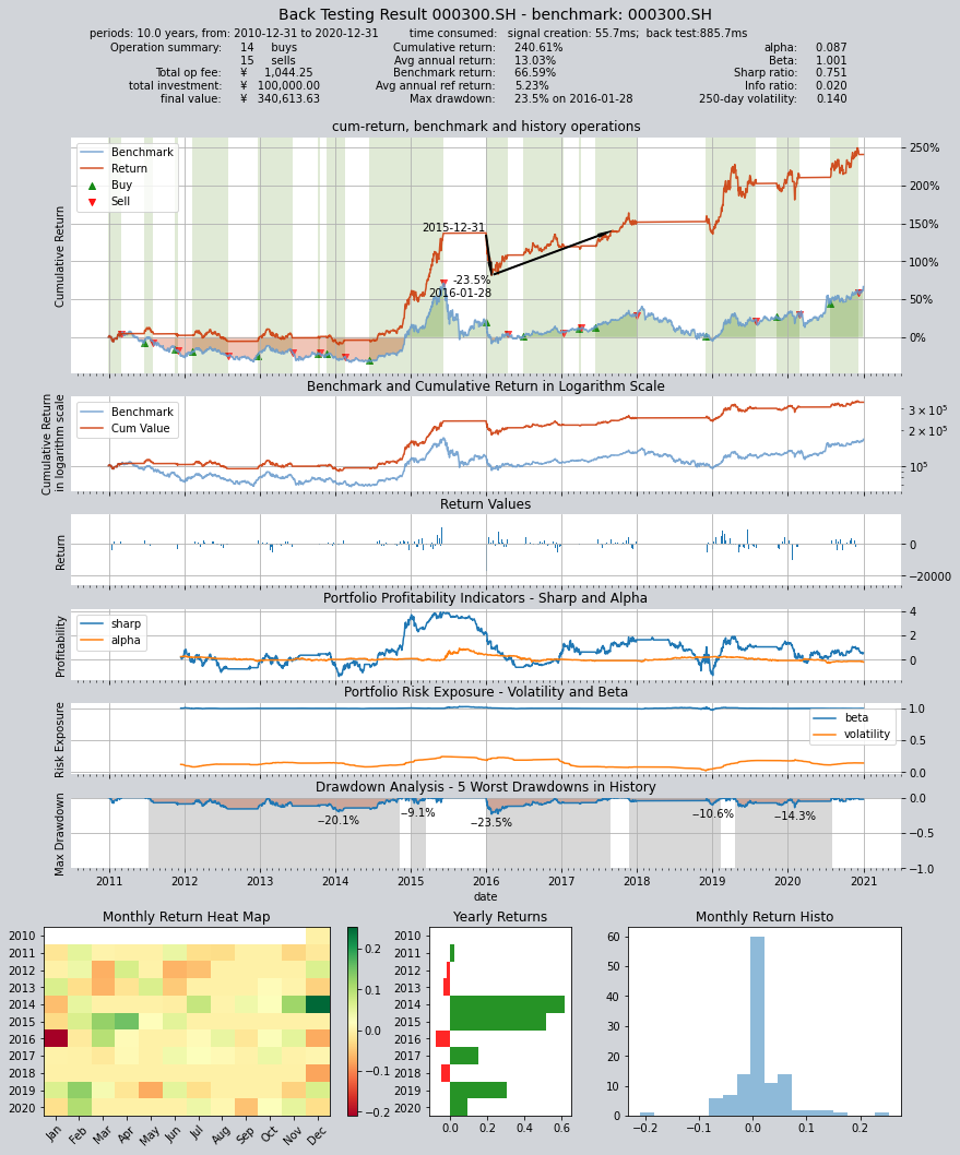
After the optimization, we can see thirty sets of best parameters, and even the worst one can achieve a final asset of over 60,000 yuan. We can manually select the best parameters from them and conduct another backtest:

We can find that the final value has skyrocketed from 19,000 in the last backtest to 124,000, with an annualized return of 18.9%, and the Sharpe ratio has also risen to 0.833

op.set_parameter('dma', pars=(104, 142, 87))
qt.run(op,
      mode=1, visual=True)

Output backtesting results are as follows:

     ====================================
     |                                  |
     |       BACK TESTING RESULT        |
     |                                  |
     ====================================

qteasy running mode: 1 - History back testing
time consumption for operate signal creation: 55.7ms
time consumption for operation back looping:  885.7ms

investment starts on      2010-12-31 00:00:00
ends on                   2020-12-31 00:00:00
Total looped periods:     10.0 years.

-------------operation summary:------------

          Sell Cnt Buy Cnt Total Long pct Short pct Empty pct
000300.SH    15       14     29   52.6%      0.0%     47.4%   

Total operation fee:     ¥    1,044.25
total investment amount: ¥  100,000.00
final value:              ¥  340,613.63
Total return:                   240.61% 
Avg Yearly return:               13.03%
Skewness:                         -0.78
Kurtosis:                         13.36
Benchmark return:                66.59% 
Benchmark Yearly return:          5.23%

------strategy loop_results indicators------ 
alpha:                            0.087
Beta:                             1.001
Sharp ratio:                      0.751
Info ratio:                       0.020
250 day volatility:               0.140
Max drawdown:                    23.53% 
    peak / valley:        2015-12-31 / 2016-01-28
    recovered on:         2017-08-28

===========END OF REPORT=============

png

Create a Custom Strategy

qteasy not only allows the use of built-in strategies, but also the creation of custom strategies. Below is a simple example that defines a simple rotation trading strategy

Back Test and evaluate Strategy

Create Strategy and Operator objects

Create Strategy object

qt.built_ins(stg_id=None)

qt.built_in_list(stg_id=None)

qt.built_in_strategies(stg_id=None)

qt.get_built_in_strategy(stg_id)

Create Operator object

qt.Operator(strategies=None, signal_type=None, op_type=None)

Three types of strategy signals

Blending Trading Signals

Get basic information of Operator object

op.info()

op.strategies

op.strategy_ids

op.strategy_count

op.signal_type

op.op_type