2. Extracting information from data tables in a standardized manner

In previous chapters, we introduced the concepts of data sources and how to populate them with financial data. In this chapter, we will explain how to extract useful information from data sources, rather than simply reading data.

QTEASY Data Management Module: 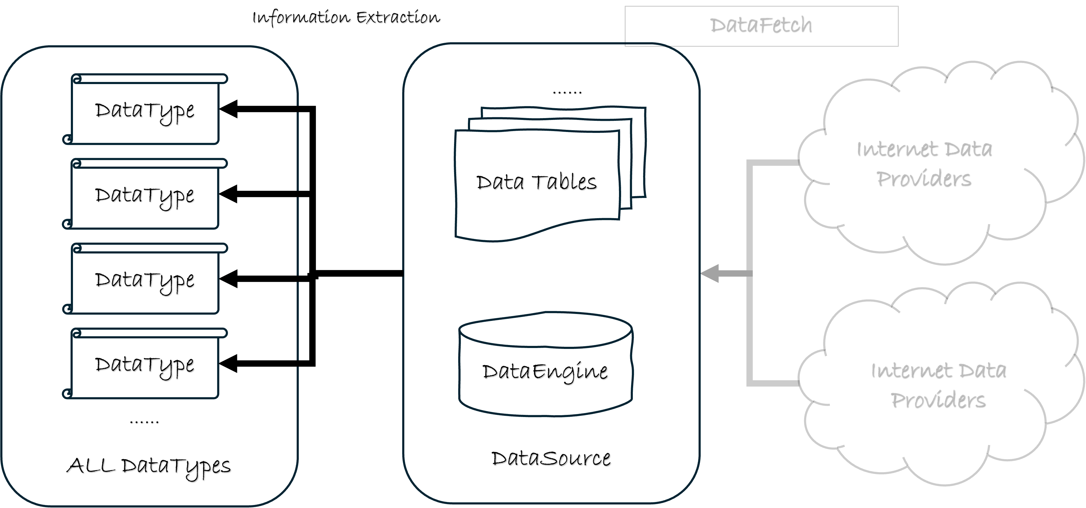Data Acquisition Module Structure

2.1. Information != Data

In quantitative trading, we need to prepare a large amount of financial data. However, the data itself is not the ultimate goal; we need to extract useful information from it. In our trading strategies, we use this information to make trading decisions.

Information is not the same as data. Some information can be directly read from data tables, such as the closing price and opening price of a stock. However, some information requires certain calculations to obtain, such as the adjusted price of a stock.

For example, in our trading strategy, we need to use the pre-adjusted price of a stock. We know that the adjusted price is calculated using the stock price and the adjustment factor, and these are stored in the following two tables:

stock_daily: A daily candlestick chart of stock prices, including information such as the opening price, closing price, highest price, and lowest price.
stock_adj_factor: This table contains information about the stock’s adjusted stock price factors.

At this point, the two tables above have stored the data we need, but they are not the information we require. We need to perform calculations to obtain the information we need.

Therefore, in order to obtain the adjusted price information, we cannot avoid the tedious calculation process.

Furthermore, it must be considered that if we need the adjusted daily candlestick price instead of the adjusted hourly candlestick price, we also need to convert the daily candlestick data to the hourly candlestick data, which makes the calculation process even more complicated.

In implementing a trading strategy, if the above conversion and calculation process is considered every time adjusted prices are used, it will make the strategy implementation complex and prone to errors. It will also cause us to scatter our limited energy on these trivial calculations instead of focusing on the strategy’s implementation.

Therefore, we need a way to encapsulate these trivial computational processes so that when implementing a strategy, we only need to focus on the strategy itself, without having to worry about these trivial computational processes.

To address this, the qteasy data management module provides a standardized way to extract information from data tables. This way is through the DataType object.

2.2. DataType object

The DataType object is an important object in the QTEASY data management module. Officially introduced in version 1.4, it encapsulates standardized data processing logic for extracting information from data tables. This allows users to define a single DataType object and focus on implementing their strategies, rather than spending time on tedious data acquisition and calculation.

qteasy provides a large number of built-in predefined DataType objects, and users can also customize DataType objects according to their own needs.

For a simple example, suppose we need to get the adjusted price of a stock after stock splits or dividends. We can directly use the built-in DataType: close|b object, as shown below:

# 获取格力电器 2025-02-01 到 2025-02-27 的后复权收盘价
import qteasy
from qteasy.datatypes import DataType

close_b = DataType(name='close|b', asset_type='E', freq='D')
# 获取数据
close_b.get_data_from_source(
        datasource=qteasy.QT_DATA_SOURCE, 
        symbols='000651.SZ', 
        starts='2025-02-01', 
        ends='2025-02-27',
)

ts_code     000651.SZ
trade_date           
2025-02-05    9234.85
2025-02-06    9194.82
2025-02-07    9295.95
2025-02-10    9245.38
2025-02-11    9199.03
2025-02-12    9220.10
2025-02-13    9232.74
2025-02-14    9268.56
2025-02-17    9201.14
2025-02-18    9066.29
2025-02-19    8836.63
2025-02-20    8817.67
2025-02-21    8714.43
2025-02-24    8695.47
2025-02-25    8533.23
2025-02-26    8621.72
2025-02-27    8729.18

2.3. List of all DataTypes (with brief descriptions)

Qteasy 2.0 includes a large number of built-in DataTypes. Each data type is uniquely identified by name, freq, and asset_type, which correspond to a specific data table and column or calculation method. A complete list can be obtained using qteasy.datatypes.get_dtype_map(), which returns a DataFrame with indices (dtype, freq, asset_type) and columns including description (purpose description), acquisition_type (acquisition method), etc.

Get the complete list

import qteasy
from qteasy import datatypes

# 仅内置类型
dtype_map = datatypes.get_dtype_map()
print(dtype_map.head(20))

# 含用户自定义类型（若有）
dtype_map_all = datatypes.get_dtype_map(include_user_defined=True)

Examples of common data types

name	freq	DataType object	Brief description of uses
trade_cal	d	None	Trading calendar
close\|b	D	E	Stock closing price after stock splits
close\|f	D	E	Stock closing price (adjusted for stock splits)
open, high, low, close, vol	D/1min/5min/…	E/IDX/FD etc.	K-line opening high low closing volume
open\|b, high\|b, etc.	D	E	Adjusted for stock splits, high and low opening prices
stock_symbol, stock_name, industry	None	E	Basic information such as stock code, name, and industry.
wt_idx\|%	d	E	Index constituent stock weighting
…	…	…	See the complete list in the output of get_dtype_map()

In the table above, common values for freq are: D for daily charts, 1min/5min for minute charts, and None for charts unrelated to frequency (e.g., basic information). asset_type: E for stocks, IDX for indices, FD for funds, and None for charts without asset restrictions. For detailed descriptions, corresponding data tables, and columns for each type, see the description and kwargs returned by get_dtype_map().

When multiple targets and data types need to be carried on the same timeline at the same time (e.g., OHLC and trading volume are included in the calculation or chart), the next chapter HistoryPanel introduces how to gather the results of get_history_data into a 3D panel; the entry point for charting can be found in the next chapter HistoryPanel Visualization.