10. Another Custom Strategy
qteasy is a fully localized deployment and operation of quantitative trading analysis toolkit, with the following functions:
Acquisition, cleaning, storage, processing, visualization, and use of financial data
Create quantitative trading strategies and provide a large number of built-in basic trading strategies
Vectorized high-speed trading strategy backtesting and trading result evaluation
Optimization and evaluation of trading strategy parameters
Deployment and live operation of trading strategies
In this tutorial, you will fully understand the main functions and usage of qteasy through a series of practical examples.
10.1. Before you start
Please make sure you have mastered the following content before starting this tutorial:
Install and configure
qteasy—— QTEASY Tutorial 1Set up a local data source, and have downloaded enough historical data to the local —
Learn to create a trader object, use built-in trading strategies —— QTEASY Tutorial 3
Learn to use the mixer to mix multiple simple strategies into more complex trading strategies —— QTEASY Tutorial 4
Learn how to customize trading strategies —— QTEASY Tutorial 5
在QTEASY文档中,还能找到更多关于使用内置交易策略、创建自定义策略等等相关内容。对qteasy的基本使用方法还不熟悉的同学,可以移步那里查看更多详细说明。
10.2. Target of this tutorial
In this section, we will continue the content of the previous section and introduce the trading strategy base class of qteasy. After introducing the simplest timing trading strategy class, we will introduce how to use the other two strategy base classes provided by qteasy to create a multi-factor stock selection strategy.
In order to provide sufficient ease of use, the various strategy base classes provided by qteasy are essentially the same, just a pre-processing form provided to reduce the user’s coding workload, and even different trading strategy base classes can be understood as “syntax sugar” designed for specific trading strategies. Therefore, the same trading strategy can often be implemented using multiple different trading strategy base classes. Therefore, in this section, we will use two different strategy base classes to implement an Alpha stock selection trading strategy.
10.3. How Alpha stock selection strategy works
The Alpha stock selection strategy we are discussing here is a low-frequency stock selection strategy that can run weekly or monthly. Each time the stock is selected, it will traverse all the constituent stocks of the HS300 index, and prioritize these 300 stocks according to certain criteria. Select the top 30 stocks from them, hold them equally, that is, rebalance the stocks once a month, sell the stocks with lower rankings during the rebalancing, buy the stocks with higher rankings, and ensure that the stocks are held in equal shares.
The ranking basis of the Alpha stock selection strategy is calculated from two financial indicators for each stock: EV (enterprise value) and EBITDA (earnings before interest, taxes, depreciation, and amortization). For each stock, compute the ratio of EV to EBITDA. When this ratio is greater than 0, it indicates that the listed company is profitable (because EBITDA is positive). In this case, the ratio represents the total enterprise value that needs to be invested for the company to earn one yuan of profit. Naturally, the lower this ratio, the better. For example, the data for the following two listed companies are as follows:
Company A has an
EBITDAof ten million, and an enterprise market value of ten billion.EV/EBITDA= 1000. This indicates that for every 1,000 yuan of the company’s market value, it can earn 1 yuan in profit.Company B also has an
EBITDAof ten million, and an enterprise market value of one hundred billion.EV/EBITDA= 10000, indicating that for every 10,000 yuan of the company’s market value, it can earn 1 yuan in profit.
Normally, we naturally feel that Company A is better because it earns the same profit with less company market value. At this time, we think that Company A’s ranking is relatively high.
According to the above rules, at the end of each month, we will rank all listed companies of the HS300 constituent stocks from small to large, and remove companies with EV/EBITDA less than 0 (of course, companies with negative profits should be removed). After that, select the top 30 companies to hold, which is the Alpha stock selection trading strategy.
In fact, for a stock-picking strategy like this that ranks by indicators, qteasy provides a built-in trading strategy that can implement it directly.
Use built_in_doc to view the documentation for this built-in trading strategy:
>>> import qteasy as qt
>>> qt.built_in_doc('finance', print_out=True)
The output is as follows:
以股票过去一段时间内的财务指标的平均值作为选股因子选股
        基础选股策略。以股票的历史指标的平均值作为选股因子,因子排序参数可以作为策略参数传入
        改变策略数据类型,根据不同的历史数据选股,选股参数可以通过pars传入
    策略参数:
        - sort_ascending: enum, 是否升序排列因子
            - True: 优先选择因子最小的股票,
            - False, 优先选择因子最大的股票
        - weighting: enum, 股票仓位分配比例权重
            - even       :默认值, 所有被选中的股票都获得同样的权重
            - linear     :权重根据因子排序线性分配
            - distance   :股票的权重与他们的指标与最低之间的差值(距离)成比例
            - proportion :权重与股票的因子分值成正比
        - condition: enum, 股票筛选条件
            - any        :默认值,选择所有可用股票
            - greater    :筛选出因子大于ubound的股票
            - less       :筛选出因子小于lbound的股票
            - between    :筛选出因子介于lbound与ubound之间的股票
            - not_between:筛选出因子不在lbound与ubound之间的股票
        - lbound: float, 股票筛选下限值, 默认值np.-inf
        - ubound: float, 股票筛选上限值, 默认值np.inf
        - max_sel_count: float, 抽取的股票的数量(p>=1)或比例(p<1), 默认值: 0.5,表示选中50%的股票
    信号类型:
        PT型: 百分比持仓比例信号
    信号规则:
        使用data_types指定一种数据类型,将股票过去的datatypes数据取平均值,将该平均值作为选股因子进行选股
    策略属性缺省值:
        默认参数: (True, 'even', 'greater', 0, 0, 0.25)
        数据类型: eps 每股收益,单数据输入
        窗口长度: 270
        参数范围: [(True, False),
        ('even', 'linear', 'proportion'),
        ('any', 'greater', 'less', 'between', 'not_between'),
        (-np.inf, np.inf),
        (-np.inf, np.inf),
        (0, 1.)]
    策略不支持参考数据,不支持交易数据
However, this built-in trading strategy only supports using qteasy built-in historical data types as stock selection factors. For example, data such as PE (price-to-earnings ratio) and profit are built-in historical data in qteasy and can be referenced directly. But if the stock selection factor cannot be found in qteasy’s built-in historical data, you cannot use the built-in trading strategy directly. The EV/EBITDA indicator is a calculated indicator, so we must use a custom trading strategy and compute this indicator within the custom strategy.
10.4. Calculate stock selection indicators
To calculate EV/EBITDA, we must at least confirm whether qteasy has provided EV and EBITDA these two types of historical data:
We can use the API: find_history_data() to check whether a historical data type is supported by qteasy. First, look up ebitda.
>>> qt.find_history_data('ebitda')
The output is as follows:
matched following history data,
use "qt.get_history_data()" to load these historical data by its data_id:
------------------------------------------------------------------------
              freq asset      table                  desc
data_id
ebitda           q     E  financial  上市公司财务指标 - 息税折旧摊销前利润
========================================================================
['income_ebitda', 'ebitda']
Data types in qteasy need to be created via qteasy.DataType. DataType represents a kind of historical data type—i.e., a category of information that qteasy can extract directly from historical data. Through data type objects, qteasy provides a unified data interface, allowing users to easily obtain various kinds of historical data without worrying about how the data type is stored or where it is stored. At the same time, qteasy fully encapsulates all the complex underlying data logic such as type handling, frequency conversion, and ticker matching, so users don’t need to care about the storage method of each kind of data and can use it directly.
关于qteasy数据类型的更详细介绍,请参见QTEASY文档。
qteasy’s DataType includes three attributes:
name: the name of the data type, for example
ebitdain the return value abovefreq: the frequency of the data, for example
qin the return value above, which represents quarterly dataasset_type: the asset type of the data; for example,
Ein the return value above represents stock data
These three attributes together define a unique data type. qteasy has a large number of built-in historical data types. Users can directly use these data types to obtain historical data, without having to calculate them themselves or process raw data to derive these data types.
From the return value above, we can see that in qteasy’s built-in historical data types, EBITDA is a standard historical data type. This data comes from the listed companies’ financial indicators table financial, and the data frequency is q (quarterly):
Next, look at EV:
>>> qt.find_history_data('ev')
The output is as follows:
matched following history data,
use "qt.get_history_data()" to load these historical data by its data_id:
------------------------------------------------------------------------
Empty DataFrame
Columns: [freq, asset_type, table_name, description]
Index: []
========================================================================
This indicates that among qteasy’s built-in historical data types, no historical data type named EV was found; in this case, you can use the parameter fuzzy=True to confirm.
>>> qt.find_history_data('ev', fuzzy=True)
The output is as follows:
matched following history data,
use "qt.get_history_data()" to load these historical data by its data_id:
------------------------------------------------------------------------
                                    name  freq asset              table               column                desc
data_id
sw_level                        sw_level  None   IDX  sw_industry_basic                level         申万行业分类 - 级别
sw_level|%                    sw_level|%  None   IDX  sw_industry_basic                level        申万行业分类筛选 - %
managers_lev                managers_lev     d     E       stk_managers                  lev       公司高管信息 - 岗位类别
total_revenue              total_revenue     q     E             income        total_revenue     上市公司利润表 - 营业总收入
revenue                          revenue     q     E             income              revenue      上市公司利润表 - 营业收入
withdra_biz_devfund  withdra_biz_devfund     q     E             income  withdra_biz_devfund  上市公司利润表 - 提取企业发展基金
express_revenue          express_revenue     q     E            express              revenue  上市公司业绩快报 - 营业收入(元)
total_revenue_ps        total_revenue_ps     q     E          financial     total_revenue_ps  上市公司财务指标 - 每股营业总收入
revenue_ps                    revenue_ps     q     E          financial           revenue_ps   上市公司财务指标 - 每股营业收入
========================================================================
The table above lists the data types that have already been defined in qteasy and can be used directly. Please pay attention to the name / freq / asset columns, which represent the data type name, data frequency, and asset type, respectively. Together, these three columns define a unique data type. Users can create a data type object via qteasy.DataType(name, freq, asset) to obtain the historical data of that data type.
Although EV is not among qteasy’s built-in historical data types, we can see that there are some historical data types related to EV, such as total revenue, earnings per share, and so on. These data types are related to EV, but they are not the EV we need.
However, we know that EV can be calculated using the following formula:
And the above financial indicators are directly supported by qteasy
Total Market Value - Data Type:
total_mvTotal Liabilities - Data Type:
total_liabTotal Cash - Data Type:
c_cash_equ_end_period
So we can test it and look at the detailed explanations of these data types:
>>> qt.find_history_data('total_mv', fuzzy=True)
You will get the following output:
matched following history data,
use "qt.get_history_data()" to load these historical data by its data_id:
------------------------------------------------------------------------
                      name freq asset             table    column                 desc
data_id
ths_total_mv  ths_total_mv    d   IDX   ths_index_daily  total_mv  同花顺指数日K线 - 总市值 (万元)
sw_total_mv    sw_total_mv    d   IDX    sw_index_daily  total_mv   申万指数日K线 - 总市值 (万元)
total_mv          total_mv    d   IDX   index_indicator  total_mv    指数技术指标 - 当日总市值(元)
total_mv          total_mv    d     E   stock_indicator  total_mv    股票技术指标 - 总市值 (万元)
total_mv_2      total_mv_2    d     E  stock_indicator2  total_mv     股票技术指标 - 总市值(亿元)
========================================================================
Note that the total_mv data type has two versions: one in units of 10,000 yuan and one in units of 100 million yuan. When calculating EV/EBITDA, strictly speaking the unit is not important, but in other cases you need to pay attention. Here we multiply this data by 10,000 to unify the units.
Here we choose DataType('total_mv', 'd', 'E'). This data type represents the total market capitalization of a listed company on each day, in units of 10,000 yuan.
>>> qt.find_history_data('total_liab', fuzzy=True)
matched following history data,
use "qt.get_history_data()" to load these historical data by its data_id:
------------------------------------------------------------------------
                                    name freq asset    table               column                   desc
data_id
total_liab                    total_liab    q     E  balance           total_liab       上市公司资产负债表 - 负债合计
total_liab_hldr_eqy  total_liab_hldr_eqy    q     E  balance  total_liab_hldr_eqy  上市公司资产负债表 - 负债及股东权益总计
========================================================================
Here we can choose the data type DataType('total_liab', 'q', 'E'). This data type represents the total liabilities of a listed company at the end of each quarter, in units of yuan.
>>> qt.find_history_data('cash', fuzzy=True)
matched following history data,
use "qt.get_history_data()" to load these historical data by its data_id:
------------------------------------------------------------------------
                                                      name freq asset      table                        column                                desc
data_id
cash_reser_cb                                cash_reser_cb    q     E    balance                 cash_reser_cb             上市公司资产负债表 - 现金及存放中央银行款项
ifc_cash_incr                                ifc_cash_incr    q     E   cashflow                 ifc_cash_incr            上市公司现金流量表 - 收取利息和手续费净增加额
oth_cash_pay_oper_act                oth_cash_pay_oper_act    q     E   cashflow         oth_cash_pay_oper_act          上市公司现金流量表 - 支付其他与经营活动有关的现金
st_cash_out_act                            st_cash_out_act    q     E   cashflow               st_cash_out_act              上市公司现金流量表 - 经营活动现金流出小计
n_cashflow_act                              n_cashflow_act    q     E   cashflow                n_cashflow_act           上市公司现金流量表 - 经营活动产生的现金流量净额
n_cashflow_inv_act                      n_cashflow_inv_act    q     E   cashflow            n_cashflow_inv_act           上市公司现金流量表 - 投资活动产生的现金流量净额
oth_cash_recp_ral_fnc_act        oth_cash_recp_ral_fnc_act    q     E   cashflow     oth_cash_recp_ral_fnc_act          上市公司现金流量表 - 收到其他与筹资活动有关的现金
stot_cash_in_fnc_act                  stot_cash_in_fnc_act    q     E   cashflow          stot_cash_in_fnc_act              上市公司现金流量表 - 筹资活动现金流入小计
free_cashflow                                free_cashflow    q     E   cashflow                 free_cashflow                上市公司现金流量表 - 企业自由现金流量
oth_cashpay_ral_fnc_act            oth_cashpay_ral_fnc_act    q     E   cashflow       oth_cashpay_ral_fnc_act          上市公司现金流量表 - 支付其他与筹资活动有关的现金
stot_cashout_fnc_act                  stot_cashout_fnc_act    q     E   cashflow          stot_cashout_fnc_act              上市公司现金流量表 - 筹资活动现金流出小计
n_cash_flows_fnc_act                  n_cash_flows_fnc_act    q     E   cashflow          n_cash_flows_fnc_act           上市公司现金流量表 - 筹资活动产生的现金流量净额
eff_fx_flu_cash                            eff_fx_flu_cash    q     E   cashflow               eff_fx_flu_cash              上市公司现金流量表 - 汇率变动对现金的影响
n_incr_cash_cash_equ                  n_incr_cash_cash_equ    q     E   cashflow          n_incr_cash_cash_equ            上市公司现金流量表 - 现金及现金等价物净增加额
c_cash_equ_beg_period                c_cash_equ_beg_period    q     E   cashflow         c_cash_equ_beg_period            上市公司现金流量表 - 期初现金及现金等价物余额
c_cash_equ_end_period                c_cash_equ_end_period    q     E   cashflow         c_cash_equ_end_period            上市公司现金流量表 - 期末现金及现金等价物余额
incl_cash_rec_saims                    incl_cash_rec_saims    q     E   cashflow           incl_cash_rec_saims     上市公司现金流量表 - 其中:子公司吸收少数股东投资收到的现金
im_net_cashflow_oper_act          im_net_cashflow_oper_act    q     E   cashflow      im_net_cashflow_oper_act      上市公司现金流量表 - 经营活动产生的现金流量净额(间接法)
im_n_incr_cash_equ                      im_n_incr_cash_equ    q     E   cashflow            im_n_incr_cash_equ       上市公司现金流量表 - 现金及现金等价物净增加额(间接法)
net_cash_rece_sec                        net_cash_rece_sec    q     E   cashflow             net_cash_rece_sec        上市公司现金流量表 - 代理买卖证券收到的现金净额(元)
cashflow_credit_impa_loss        cashflow_credit_impa_loss    q     E   cashflow              credit_impa_loss                  上市公司现金流量表 - 信用减值损失
end_bal_cash                                  end_bal_cash    q     E   cashflow                  end_bal_cash                 上市公司现金流量表 - 现金的期末余额
beg_bal_cash                                  beg_bal_cash    q     E   cashflow                  beg_bal_cash               上市公司现金流量表 - 减:现金的期初余额
end_bal_cash_equ                          end_bal_cash_equ    q     E   cashflow              end_bal_cash_equ            上市公司现金流量表 - 加:现金等价物的期末余额
beg_bal_cash_equ                          beg_bal_cash_equ    q     E   cashflow              beg_bal_cash_equ            上市公司现金流量表 - 减:现金等价物的期初余额
cash_ratio                                      cash_ratio    q     E  financial                    cash_ratio                   上市公司财务指标 - 保守速动比率
salescash_to_or                            salescash_to_or    q     E  financial               salescash_to_or       上市公司财务指标 - 销售商品提供劳务收到的现金/营业收入
cash_to_liqdebt                            cash_to_liqdebt    q     E  financial               cash_to_liqdebt                上市公司财务指标 - 货币资金/流动负债
cash_to_liqdebt_withinterest  cash_to_liqdebt_withinterest    q     E  financial  cash_to_liqdebt_withinterest              上市公司财务指标 - 货币资金/带息流动负债
q_salescash_to_or                        q_salescash_to_or    q     E  financial             q_salescash_to_or  上市公司财务指标 - 销售商品提供劳务收到的现金/营业收入(单季度)
cash_div_planned                          cash_div_planned    d     E   dividend                      cash_div                         预案-每股分红(税后)
cash_div_tax_planned                  cash_div_tax_planned    d     E   dividend                  cash_div_tax                         预案-每股分红(税前)
cash_div_approved                        cash_div_approved    d     E   dividend                      cash_div                     股东大会批准-每股分红(税后)
cash_div_tax_approved                cash_div_tax_approved    d     E   dividend                  cash_div_tax                     股东大会批准-每股分红(税前)
cash_div                                          cash_div    d     E   dividend                      cash_div                         实施-每股分红(税后)
cash_div_tax                                  cash_div_tax    d     E   dividend                  cash_div_tax                         实施-每股分红(税前)
========================================================================
There are many data types related to cash, but the total cash and cash equivalents we need is DataType(c_cash_equ_end_period, 'q', 'E'). This data type represents the total cash and cash equivalents of a listed company at the end of each quarter.
Based on the information above, we can choose the following four data types to calculate EV:
DataType('total_mv', 'd', 'E'), this data type represents the total market capitalization of a listed company on each day, in units of 10,000 yuan.DataType('total_liab', 'q', 'E'): this data type represents a listed company’s total liabilities at the end of each quarter, in yuan.DataType('c_cash_equ_end_period', 'q', 'E'): this data type represents a listed company’s total cash and cash equivalents at the end of each quarter, in yuan.
We can run a quick test. qteasy provides a very convenient API: get_history_data(), which can directly retrieve historical data for these data types:
# 创建数据类型对象
dtypes = [DataType('total_mv', freq='d', asset_type='E'),
          DataType('total_liab', freq='q', asset_type='E'),
          DataType('c_cash_equ_end_period', freq='q', asset_type='E'),
          DataType('ebitda', freq='q', asset_type='E')]
# 获取沪深300指数成分股(这里只获取前20支股票)
shares = qt.filter_stock_codes(index='000300.SH', date='20220131')[:20]
# 获取所有股票的总市值、总负债、总现金、EBITDA数据
dt = qt.get_history_data(data_types=dtypes, shares=shares, asset_type='any', freq='m')
# 随便选择一支股票,转化为DataFrame检查数据是否正确获取
one_share = shares[1]
df = dt[one_share]
# 计算EV/EBITDA选股因子
df['ev_to_ebitda'] = (df.total_mv + df.total_liab - df.c_cash_equ_end_period) / df.ebitda
print(df)
                total_mv    total_liab  c_cash_equ_end_period        ebitda  \
2022-01-04  2.382041e+07           NaN                    NaN           NaN
2022-01-05  2.461094e+07           NaN                    NaN           NaN
2022-01-06  2.447143e+07           NaN                    NaN           NaN
2022-01-07  2.544796e+07           NaN                    NaN           NaN
2022-01-10  2.576185e+07           NaN                    NaN           NaN
...                  ...           ...                    ...           ...
2022-12-26  2.136561e+07  1.426656e+12           1.158051e+11  2.969171e+10
2022-12-27  2.152844e+07  1.426656e+12           1.158051e+11  2.969171e+10
2022-12-28  2.160986e+07  1.426656e+12           1.158051e+11  2.969171e+10
2022-12-29  2.112137e+07  1.426656e+12           1.158051e+11  2.969171e+10
2022-12-30  2.116789e+07  1.426656e+12           1.158051e+11  2.969171e+10

            ev_to_ebitda
2022-01-04           NaN
2022-01-05           NaN
2022-01-06           NaN
2022-01-07           NaN
2022-01-10           NaN
...                  ...
2022-12-26     51.344518
2022-12-27     51.399358
2022-12-28     51.426778
2022-12-29     51.262258
2022-12-30     51.277926

[242 rows x 5 columns]
We can see that the stock selection factor has been calculated, so we can start defining the trading strategy.
10.5. Define Alpha stock selection strategy with FactorSorter
qteasy provides the FactorSorter trading strategy class for this type of timed stock selection trading strategy. As the name suggests, this trading strategy base class allows users to calculate a set of stock selection factors in the implementation method of the strategy, so that the strategy can automatically sort all stocks according to the value of the stock selection factor, and select the stocks with higher rankings. As for the sorting method, screening rules, stock holding weights, etc., can be set through strategy parameters.
If it meets the definition of the trading strategy above, using the FactorSorter strategy base class will be very convenient.
Next, let’s define it step by step. First, inherit FactorSorter and define a class. In the previous section, we defined the name, description, default parameters, and other information in the __init__() method of the custom strategy. However, we can also ignore the __init__() method and only pass in parameters when creating the strategy object. This is also possible. We do it here:
>>> class AlphaFac(qt.FactorSorter):  # 注意这里使用FactorSorter策略类
...
...     def realize(self):
...         # 从历史数据编码中读取四种历史数据的最新数值
...         total_mv = self.get_data('total_mv_E_d')[-1]  # 总市值
...         total_liab = self.get_data('total_liab_E_q')[-1]  # 总负债
...         cash_equ = self.get_data('c_cash_equ_end_period_E_q')[-1]  # 现金及现金等价物总额
...         ebitda = self.get_data('ebitda_E_q')[-1]  # ebitda,息税折旧摊销前利润
...         # 选股因子为EV/EBIDTA,使用下面公式计算
...         factor = (total_mv * 10000 + total_liab - cash_equ) / ebitda
...         return factor  # 直接返回选股因子,策略就定义好了
Same as in the previous section, the first step in realize() is to fetch historical data. We know the historical data includes four types: total_mv, total_liab, c_cash_equ_end_period, ebitda. These four historical data series will be defined as four DataTypes and passed into the strategy. To use these historical data in the strategy, you can directly call self.get_data():
# 从历史数据编码中读取四种历史数据的最新数值
total_mv = self.get_data('total_mv_E_d')[-1]  # 总市值
total_liab = self.get_data('total_liab_E_q'))[-1]  # 总负债
cash_equ = self.get_data('c_cash_equ_end_period_E_q'))[-1]  # 现金及现金等价物总额
ebitda = self.get_data('ebitda_E_q'))[-1]  # ebitda,息税折旧摊销前利润
        ...
The self.get_data() method retrieves the corresponding historical data via each data item’s data ID. By default, the ID of each data item is a combination of its name, asset type, and frequency, for example:
DataType('total_mv', 'd', 'E'): the ID of this data type istotal_mv_E_d.DataType('total_liab', 'q', 'E'): the ID of this data type is:total_liab_E_d.
Before the trading strategy starts running, qteasy will prepare the corresponding trading data. All trading data are stored in a numpy array: the number of columns corresponds to the number of stocks in the universe, and each column corresponds to one stock in the universe; the number of rows corresponds to the length of the time window, each row corresponds to a time point in the time window and is sorted in ascending order, and the last column represents the latest historical data visible at the time of trading.
Following this rule, to get the most recent historical data that can be seen on the trading day for the i-th stock, just access array(-1, i). With the loop below, you can access the data for all stocks at the same point in time:
total_mv = self.get_data('total_mv_E_d')
# 循环访问每一支股票的total_mv
for i in len(total_mv[-1]):
    print(f'total mv of share {i}: {total_mv[-1, i]}')
However, using a for-loop to access data is relatively inefficient. You should use vectorized operations as much as possible in your strategy to save time.
If you are ready for the above, it is very convenient to calculate the stock selection factor. Moreover, since we use the FactorSorter strategy base class, after calculating the stock selection factor, you can directly return the stock selection factor, and qteasy will handle the rest of the stock selection operation:
# 选股因子为EV/EBIDTA,使用下面公式计算
factor = (total_mv * 10000 + total_liab - cash_equ) / ebitda
return factor  # 直接返回选股因子,策略就定义好了
Now, with just six lines of code, a custom Alpha stock selection trading strategy is defined. Isn’t it very simple?
OK, let’s see how the backtest results are?
10.6. Results of backtesting trading strategies
Since we ignored the __init__() method of the strategy class, the complete strategy parameters must be entered when instantiating the strategy object:
>>> from qteasy import Parameter, StgData

>>> alpha = AlphaFac(
...     pars=[],
...     name='AlphaSel',
...     description='本策略每隔1个月定时触发计算SHSE.000300成份股的过去的EV/EBITDA并选取EV/EBITDA大于0的股票',
...     data_types=[DataType('total_mv', freq='d', asset_type='E'),
...                 DataType('total_liab', freq='q', asset_type='E'),
...                 DataType('c_cash_equ_end_period', freq='q', asset_type='E'),
...                 DataType('ebitda', freq='q', asset_type='E')],
...     window_length=[20, 20, 10, 10],  # 现在可以为每一种数据类型设置不同的窗口长度
...     max_sel_count=30,  # 设置选股数量,最多选出30个股票
...     condition='greater',  # 设置筛选条件,仅筛选因子大于ubound的股票
...     ubound=0.0,  # 设置筛选条件,仅筛选因子大于0的股票
...     weighting='even',  # 设置股票权重,所有选中的股票平均分配权重
...     sort_ascending=True,  # 设置排序方式,因子从小到大排序选择头30名
... )
Then create an Operator object, because we want to control the position ratio, it is best to use the ‘PT’ signal type:
>>> op = qt.Operator(alpha, signal_type='PT')
>>> res = op.run(mode=1,
...        asset_type='E',
...        asset_pool=shares,
...        PT_buy_threshold=0.0,
...        PT_sell_threshold=0.0,
...        trade_batch_size=100,
...        sell_batch_size=1)
Results of backtesting:
     ====================================
     |                                  |
     |       BACK TESTING RESULT        |
     |                                  |
     ====================================

qteasy running mode: 1 - History back testing
time consumption for operate signal creation: 9.4ms
time consumption for operation back looping:  5s 831.0ms

investment starts on      2016-04-05 00:00:00
ends on                   2021-02-01 00:00:00
Total looped periods:     4.8 years.

-------------operation summary:------------
Only non-empty shares are displayed, call
"loop_result["oper_count"]" for complete operation summary

          Sell Cnt Buy Cnt Total Long pct Short pct Empty pct
000301.SZ    1        2       3   10.3%      0.0%     89.7%
000786.SZ    2        3       5   27.5%      0.0%     72.5%
000895.SZ    1        0       1   62.6%      0.0%     37.4%
002001.SZ    2        2       4   55.8%      0.0%     44.2%
002007.SZ    3        1       4   68.3%      0.0%     31.7%
002027.SZ    2        9      11   41.3%      0.0%     58.7%
002032.SZ    2        0       2    5.9%      0.0%     94.1%
002044.SZ    1        1       2    1.8%      0.0%     98.2%
002049.SZ    1        1       2    5.1%      0.0%     94.9%
002050.SZ    4        5       9   13.8%      0.0%     86.2%
...            ...     ...   ...      ...       ...       ...
603517.SH    1        1       2    1.8%      0.0%     98.2%
603806.SH    6        3       9   39.8%      0.0%     60.2%
603899.SH    1        1       2   31.0%      0.0%     69.0%
000408.SZ    3        6       9   35.5%      0.0%     64.5%
002648.SZ    1        1       2    5.2%      0.0%     94.8%
002920.SZ    1        1       2    1.7%      0.0%     98.3%
300223.SZ    1        1       2    5.2%      0.0%     94.8%
600219.SH    1        1       2    6.1%      0.0%     93.9%
603185.SH    1        1       2    5.2%      0.0%     94.8%
688005.SH    1        1       2    5.2%      0.0%     94.8%

Total operation fee:     ¥      928.22
total investment amount: ¥  100,000.00
final value:              ¥  159,072.14
Total return:                    59.07%
Avg Yearly return:               10.09%
Skewness:                         -0.28
Kurtosis:                          3.29
Benchmark return:                65.96%
Benchmark Yearly return:         11.06%

------strategy loop_results indicators------
alpha:                           -0.012
Beta:                             1.310
Sharp ratio:                      1.191
Info ratio:                      -0.010
250 day volatility:               0.105
Max drawdown:                    20.49%
    peak / valley:        2018-05-22 / 2019-01-03
    recovered on:         2019-12-26

===========END OF REPORT=============
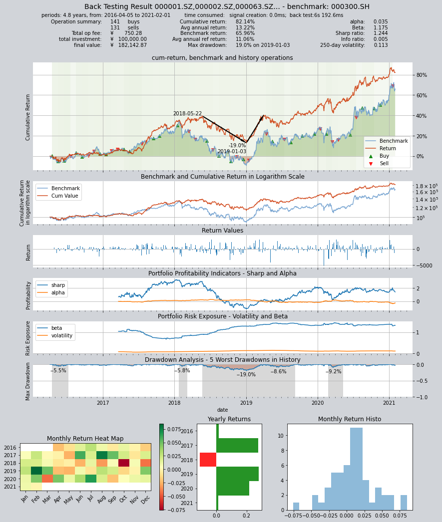
Backtesting results show that this strategy cannot effectively outperform the Shanghai and Shenzhen 300 Index, but overall, the drawdown is relatively small and the risk is low, making it a good bottom strategy.
But the performance of the strategy is not the focus of our discussion. Next, let’s take a look at how to define the same Alpha stock selection strategy without using the FactorSorter base class.
10.7. Define an Alpha stock selection strategy with GeneralStg
We have introduced two strategy base classes before:
RuleIterator: Users only need to define stock selection rules for a stock, andqteasywill apply the same rules to all stocks in the stock pool, and can also set different adjustable parameters for different stocksFactorSorter:Users only need to define a stock selection factor, andqteasywill automatically select the best stocks to hold based on the stock selection factor after sorting, and sell the stocks that are not qualified.
While GeneralStg is a basic strategy base class provided by qteasy, it does not provide any “syntax sugar” functions to help users reduce coding workload, but precisely because it does not have syntax sugar, it is a real “universal” strategy class that can be used to create trading strategies more freely.
Above Alpha stock selection trading strategy can be easily implemented with FactorSorter, but to understand GeneralStg, let’s see how to use it to create the same strategy:
Here is the complete code:
class AlphaPT(qt.GeneralStg):

    def realize(self, h, r=None, t=None, pars=None):

        # 从历史数据编码中读取四种历史数据的最新数值
        total_mv = h[:, -1, 0]  # 总市值
        total_liab = h[:, -1, 1]  # 总负债
        cash_equ = h[:, -1, 2]  # 现金及现金等价物总额
        ebitda = h[:, -1, 3]  # ebitda,息税折旧摊销前利润

        # 选股因子为EV/EBIDTA,使用下面公式计算
        factors = (total_mv + total_liab - cash_equ) / ebitda
        # 处理交易信号,将所有小于0的因子变为NaN
        factors = np.where(factors < 0, np.nan, factors)
        # 选出数值最小的30个股票的序号
        arg_partitioned = factors.argpartition(30)
        selected = arg_partitioned[:30]  # 被选中的30个股票的序号
        not_selected = arg_partitioned[30:]  # 未被选中的其他股票的序号(包括因子为NaN的股票)

        # 开始生成PT交易信号
        signal = np.zeros_like(factors)
        # 所有被选中的股票的持仓目标被设置为0.03,表示持有3.3%
        signal[selected] = 0.0333
        # 其余未选中的所有股票持仓目标在PT信号模式下被设置为0,代表目标仓位为0
        signal[not_selected] = 0

        return signal
Compare the above code with the code of FactorSorter, you can find that the code of GeneralStg has more factor processing work after calculating the stock selection factor:
Remove factors less than zero
Sort and select the smallest 30 of the remaining factors
Set the position ratio of the selected stocks to 3.3%
In fact, all of the above work is the “syntax sugar” provided by FactorSorter, which we must manually implement here. It is worth noting that the sorting and other codes I used in the above examples are highly optimized numpy codes directly extracted from FactorSorter, and their running speed is very fast, much faster than the code that general users can write. Therefore, as long as the conditions permit, users should try to use these syntax sugars as much as possible, and only write sorting code when necessary.
You may study the above code, but please note that if you use the GeneralStg strategy class, the output of the strategy should be the target position of the stock, not the stock selection factor.
Here is the backtesting results:
10.8. Backtesting results:
Backtesting with the same data:
alpha = AlphaPT(pars=(),
                 par_count=0,
                 par_types=[],
                 par_range=[],
                 name='AlphaSel',
                 description='本策略每隔1个月定时触发计算SHSE.000300成份股的过去的EV/EBITDA并选取EV/EBITDA大于0的股票',
                 data_types='total_mv, total_liab, c_cash_equ_end_period, ebitda',
                 run_freq='m',
                 data_freq='d',
                 window_length=100)
op = qt.Operator(alpha, signal_type='PT')
res = op.run(mode=1,
             asset_type='E',
             asset_pool=shares,
             PT_buy_threshold=0.00,  # 如果设置PBT=0.00,PST=0.03,最终收益会达到30万元
             PT_sell_threshold=0.00,
             trade_batch_size=100,
             sell_batch_size=1,
             trade_log=True
            )
Results of backtesting:
     ====================================
     |                                  |
     |       BACK TESTING RESULT        |
     |                                  |
     ====================================

qteasy running mode: 1 - History back testing
time consumption for operate signal creation: 7.2ms
time consumption for operation back looping:  6s 308.5ms

investment starts on      2016-04-05 00:00:00
ends on                   2021-02-01 00:00:00
Total looped periods:     4.8 years.

-------------operation summary:------------
Only non-empty shares are displayed, call
"loop_result["oper_count"]" for complete operation summary

          Sell Cnt Buy Cnt Total Long pct Short pct Empty pct
000301.SZ    1        1       2   10.3%      0.0%     89.7%
000786.SZ    2        3       5   27.5%      0.0%     72.5%
000895.SZ    1        1       2   68.7%      0.0%     31.3%
002001.SZ    2        2       4   57.5%      0.0%     42.5%
002007.SZ    0        1       1   68.3%      0.0%     31.7%
002027.SZ    6        7      13   41.3%      0.0%     58.7%
002032.SZ    3        1       4    7.5%      0.0%     92.5%
002044.SZ    1        1       2    1.8%      0.0%     98.2%
002049.SZ    1        1       2    5.1%      0.0%     94.9%
002050.SZ    4        4       8   13.8%      0.0%     86.2%
...            ...     ...   ...      ...       ...       ...
603806.SH    5        3       8   62.1%      0.0%     37.9%
603899.SH    2        3       5   36.3%      0.0%     63.7%
000408.SZ    3        5       8   35.5%      0.0%     64.5%
002648.SZ    1        1       2    5.2%      0.0%     94.8%
002920.SZ    1        1       2    5.1%      0.0%     94.9%
300223.SZ    1        2       3    5.2%      0.0%     94.8%
300496.SZ    1        1       2   10.5%      0.0%     89.5%
600219.SH    1        1       2    6.1%      0.0%     93.9%
603185.SH    1        1       2    5.2%      0.0%     94.8%
688005.SH    1        2       3    5.2%      0.0%     94.8%

Total operation fee:     ¥      985.25
total investment amount: ¥  100,000.00
final value:              ¥  189,723.44
Total return:                    89.72%
Avg Yearly return:               14.18%
Skewness:                         -0.41
Kurtosis:                          2.87
Benchmark return:                65.96%
Benchmark Yearly return:         11.06%

------strategy loop_results indicators------
alpha:                            0.044
Beta:                             1.134
Sharp ratio:                      1.284
Info ratio:                       0.011
250 day volatility:               0.120
Max drawdown:                    20.95%
    peak / valley:        2018-05-22 / 2019-01-03
    recovered on:         2019-09-09

===========END OF REPORT=============
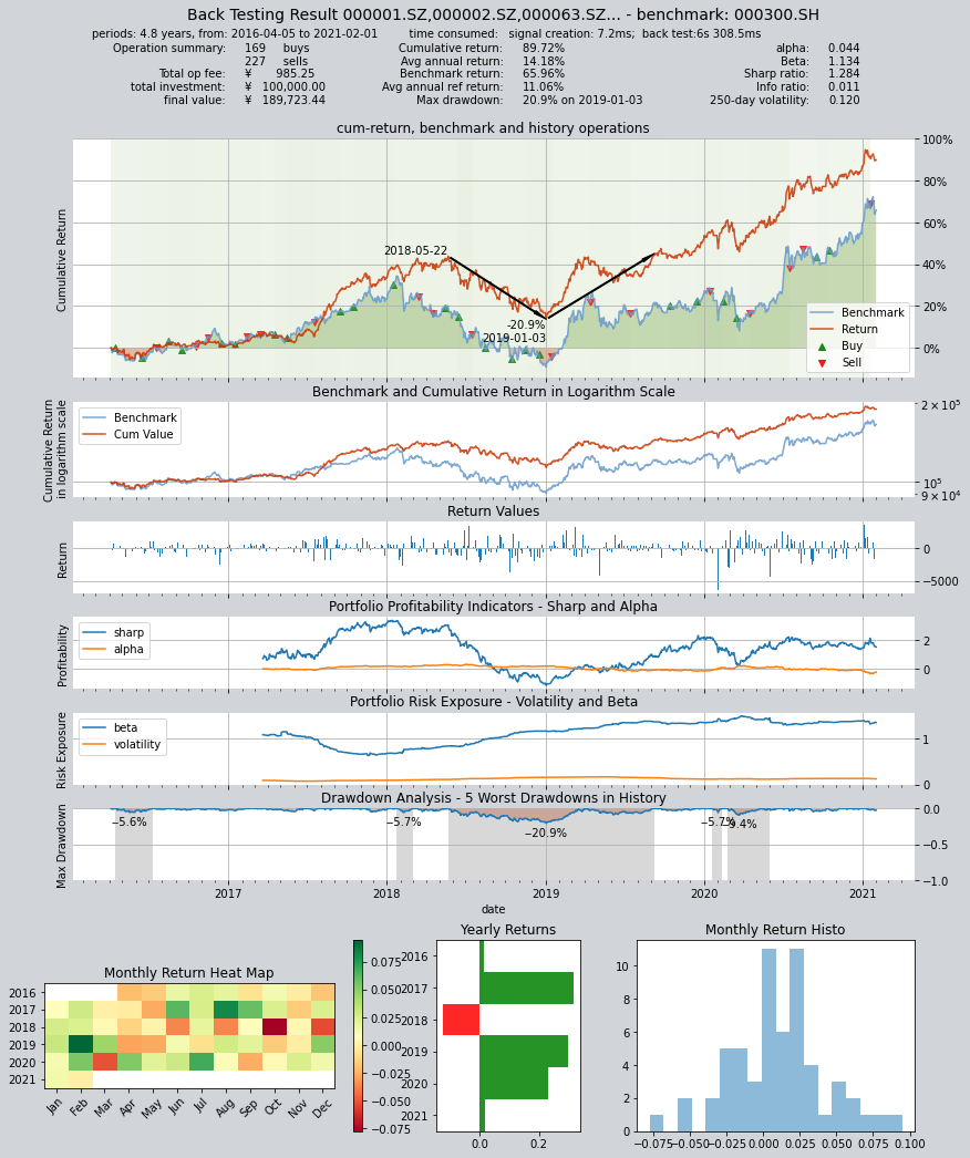
Results of the two trading strategies are basically the same
10.9. Recap
We have learned the usage of the other two trading strategy base classes FactorSorter and GeneralStg provided by qteasy in this section, and actually created two trading strategies. Although different base classes are used, the same Alpha stock selection trading strategy is created.
In the next section, we will continue to introduce custom trading strategies, but will use a more complex example to demonstrate the usage of custom trading strategies. Stay tuned!