5. Estrategia comercial pseudo-grid
Fuente de referencia: docs/_joinquant_migration_source/Example_05_Class Grid Trading.ipynb Primera celda de Markdown.
Esta estrategia primero calcula la media y la desviación estándar de los últimos 300 puntos de datos de precios (el número de días es un parámetro ajustable).
Los límites del intervalo de la cuadrícula se obtienen sumando o restando 1 y 2 desviaciones estándar de la media (el multiplicador para sumar o restar desviaciones estándar es un parámetro ajustable).
Se les asignan pesos de posición de 0,3 y 0,5 respectivamente (los pesos de posición son parámetros ajustables).
Luego, configure el tamaño de la posición según el rango de precios (+/-40 es el límite superior e inferior, lo cual no tiene significado práctico): (-40,-3],(-3,-2],(-2,2],(2,3],(3,40] (el precio específico es igual a la media más un múltiplo de la desviación estándar) [-0.5, -0.3, 0.0, 0.3, 0.5] (ratio de capital; el signo negativo aquí indica abrir una posición corta y está configurado para permitir mantener posiciones cortas durante el backtesting).
Los datos del backtesting constan de puntos de datos de 1 minuto para el índice HS300. El periodo de backtesting es desde las 09:30:00 horas del 1 de marzo de 2022 hasta las 15:00:00 horas del 31 de julio de 2022.
import qteasy as qt
print(qt.__version__)
5.1. Definir la estrategia comercial
import numpy as np
from qteasy import Parameter, StgData


class GridTrading(qt.GeneralStg):

    def __init__(self):
        super().__init__(
            name='GridTrading',
            description='根据过去窗口的均值和标准差分档生成目标仓位',
            pars=[
                Parameter((0.5, 3.0), name='low_th', par_type='float', value=2.0),
                Parameter((2.0, 8.0), name='high_th', par_type='float', value=3.0),
                Parameter((0.01, 0.6), name='low_pos', par_type='float', value=0.3),
                Parameter((0.1, 1.0), name='high_pos', par_type='float', value=0.5),
                Parameter((60, 500), name='lookback', par_type='int', value=300),
            ],
            data_types=StgData('close', freq='1min', asset_type='ANY', window_length=500),
            use_latest_data_cycle=False,
        )

    def realize(self):
        low_th, high_th, low_pos, high_pos, lookback = self.get_pars(
            'low_th', 'high_th', 'low_pos', 'high_pos', 'lookback'
        )
        close = self.get_data('close_ANY_1min')
        close = close[-lookback:]
        close_mean = np.nanmean(close, axis=0)
        close_std = np.nanstd(close, axis=0)
        current_close = close[-1]
        hi_positive = close_mean + high_th * close_std
        low_positive = close_mean + low_th * close_std
        low_negative = close_mean - low_th * close_std
        hi_negative = close_mean - high_th * close_std
        pos = np.zeros_like(close_mean, dtype=float)
        pos = np.where(current_close > hi_positive, high_pos, pos)
        pos = np.where((current_close <= hi_positive) & (current_close > low_positive), low_pos, pos)
        pos = np.where((current_close <= low_positive) & (current_close > low_negative), 0.0, pos)
        pos = np.where((current_close <= low_negative) & (current_close > hi_negative), -low_pos, pos)
        pos = np.where(current_close <= hi_negative, -high_pos, pos)
        return pos
5.2. Defina el objeto comercial, configure los ajustes comerciales y realice pruebas retrospectivas comerciales.
alpha = GridTrading()
op = qt.Operator(alpha, signal_type='PT')
op.op_type = 'batch'
op.set_blender("1.0*s0")
res = qt.run(op,
        mode=1,
        invest_start='20220401',
        invest_end='20220731',
        invest_cash_amounts=[1000000],
        asset_type='IDX',
        asset_pool=['000300.SH'],
        trade_batch_size=0.01,
        sell_batch_size=0.01,
        trade_log=True,
        allow_sell_short=True,
)
====================================
| |
| BACK TESTING RESULT |
| |
====================================
qteasy running mode: 1 - History back testing
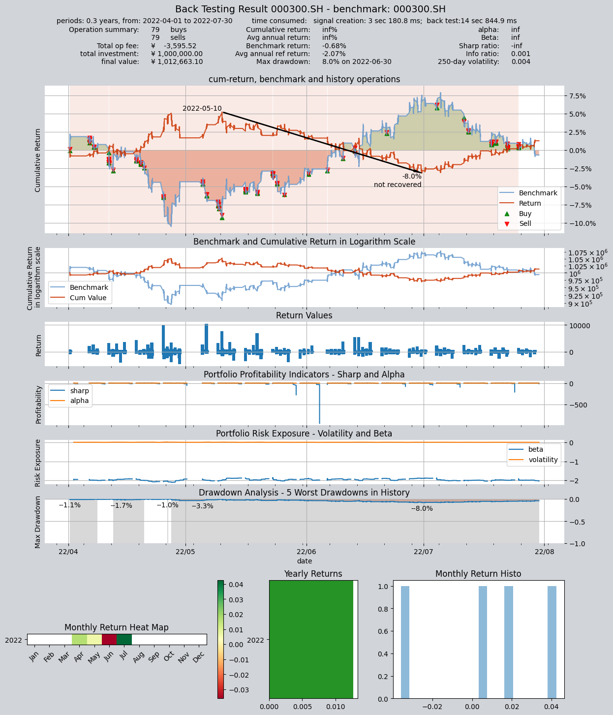
time consumption for operate signal creation: 3 sec 180.8 ms
time consumption for operation back looping: 14 sec 844.9 ms
investment starts on 2022-04-01 09:30:00
ends on 2022-07-30 15:00:00
Total looped periods: 0.3 years.
-------------operation summary:------------
Only non-empty shares are displayed, call
"loop_result["oper_count"]" for complete operation summary
Sell Cnt Buy Cnt Total Long pct Short pct Empty pct
000300.SH 79 79 158 0.0% 98.1% 1.9%
Total operation fee: ¥ -3,595.52
total investment amount: ¥1,000,000.00
final value: ¥1,012,663.10
Total return: inf%
Avg Yearly return: inf%
Skewness: 3.34
Kurtosis: 116.90
Benchmark return: -0.68%
Benchmark Yearly return: -2.07%
------strategy loop_results indicators------
alpha: inf
Beta: inf
Sharp ratio: -inf
Info ratio: 0.001
250 day volatility: 0.004
Max drawdown: 7.95%
peak / valley: 2022-05-10 / 2022-06-30
recovered on: Not recovered!
===========END OF REPORT=============