4. Selección de acciones multifactorial
Fuente de referencia: docs/_joinquant_migration_source/Example_04_Multifactor Stock Selection.ipynb Primera celda de Markdown.
Esta estrategia se activa mensualmente, realizando análisis de regresión sobre cada acción utilizando el modelo de tres factores de Fama-French para obtener su valor alfa. Suponiendo que el modelo de tres factores de Fama-French pueda explicar completamente el mercado, un alfa negativo indica que el mercado infravalora la acción, lo que justifica una compra.
Estrategia y enfoque:
Se calcularon el rendimiento de mercado, la relación libro-mercado y la capitalización de mercado de acciones individuales, y se clasificaron las dos últimas. Con base en las carteras categorizadas, se calculó su rendimiento ponderado por capitalización de mercado, SMB y HML. Se realizó una regresión en cada acción (asumiendo una tasa de rendimiento libre de riesgo de 0) para obtener el valor alfa.
Las 10 acciones con los valores alfa más bajos (menos de 0) se seleccionan para su inclusión en el grupo objetivo. Las acciones que no están en el grupo objetivo se eliminan y las acciones restantes en el grupo objetivo se compran con la misma ponderación.
Datos de backtesting: acciones constituyentes SHSE.000300
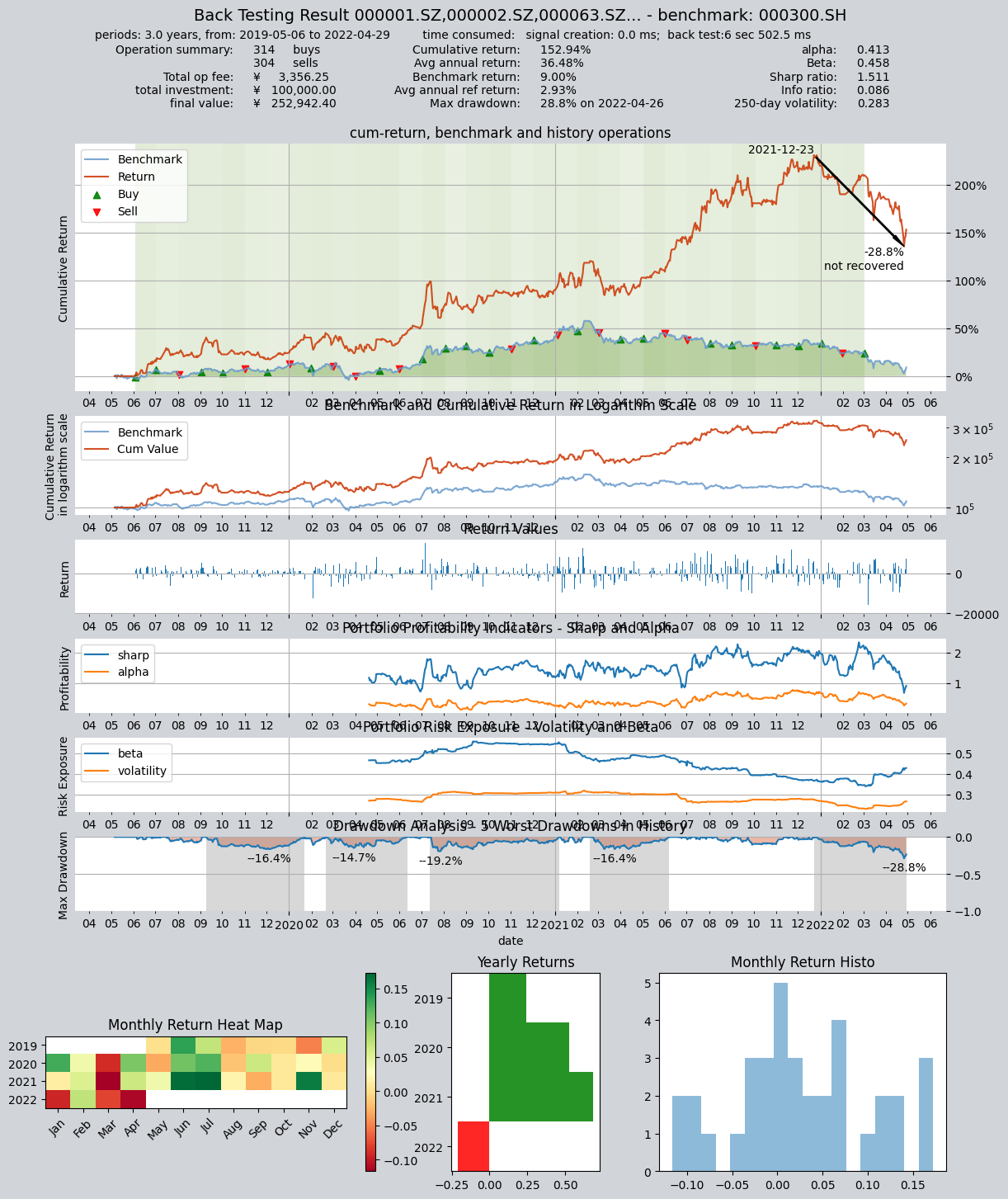
El período de backtesting fue del 1 de mayo de 2019 al 1 de mayo de 2022.
4.1. Definir estrategia
import qteasy as qt
import numpy as np
from qteasy import Parameter, StgData
def market_value_weighted(stock_return, mv, mv_cat, bp_cat, mv_target, bp_target):
    """ 根据mv_target和bp_target计算市值加权收益率

    """
    sel = (mv_cat == mv_target) & (bp_cat == bp_target)
    mv_total = np.nansum(mv[sel])
    mv_weight = mv / mv_total
    return_total = np.nansum(stock_return[sel] * mv_weight[sel])
    return return_total


class MultiFactors(qt.FactorSorter):

    def __init__(self, pars: tuple = (0.5, 0.3, 0.7)):
        super().__init__(
                name='MultiFactor',
                description='根据Fama-French三因子回归模型估算HS300成分股的alpha值选股',
                pars=[Parameter((0.01, 0.99), par_type='float', name='size_gate', value=0.5),  # 参数1:大小市值分类界限
                      Parameter((0.01, 0.49), par_type='float', name='pb_s', value=0.3),  # 参数2:小/中bp分界线
                      Parameter((0.50, 0.99), par_type='float', name='pb_l', value=0.7)],  # 参数3,中/大bp分界线
                data_types=[StgData('pb', freq='d', asset_type='E', window_length=20, use_latest_data_cycle=True),
                            StgData('total_mv', freq='d', asset_type='E', window_length=2, use_latest_data_cycle=True),
                            StgData('close', freq='d', asset_type='E', window_length=20, use_latest_data_cycle=True),
                            StgData('close-000300.SH', freq='d', asset_type='IDX', window_length=20, use_latest_data_cycle=True)],  # 执行选股需要用到的股票数据
                max_sel_count=10,  # 最多选出10支股票
                sort_ascending=True,  # 选择因子最小的股票
                condition='less',  # 仅选择因子小于某个值的股票
                lbound=0,  # 仅选择因子小于0的股票
                ubound=0,  # 仅选择因子小于0的股票
        )

    def realize(self):

        size_gate_percentile, bp_small_percentile, bp_large_percentile = self.get_pars('size_gate', 'pb_s', 'pb_l')
        # 读取投资组合的数据PB和total_MV的最新值
        pb, mv, closes, market_closes = self.get_data('pb_E_d', 'total_mv_E_d', 'close_E_d', 'close-000300.SH_IDX_d')
        pb = pb[-1]  # 当前所有股票的PB值
        mv = mv[-1]  # 当前所有股票的市值
        pre_close = closes[-2]  # 当前所有股票的前收盘价
        close = closes[-1]  # 当前所有股票的最新收盘价

        # 读取参考数据(r)
        market_pre_close = market_closes[-2]  # HS300的昨收价
        market_close = market_closes[-1]  # HS300的收盘价

        # 计算账面市值比,为pb的倒数
        bp = pb ** -1
        # 计算市值的50%的分位点,用于后面的分类
        size_gate = np.nanquantile(mv, size_gate_percentile)
        # 计算账面市值比的30%和70%分位点,用于后面的分类
        bm_30_gate = np.nanquantile(bp, bp_small_percentile)
        bm_70_gate = np.nanquantile(bp, bp_large_percentile)
        # 计算每只股票的当日收益率
        stock_return = pre_close / close - 1

        # 根据每只股票的账面市值比和市值,给它们分配bp分类和mv分类
        # 市值小于size_gate的cat为1,否则为2
        mv_cat = np.ones_like(mv)
        mv_cat += (mv > size_gate).astype('float')
        # bp小于30%的cat为1,30%~70%之间为2,大于70%为3
        bp_cat = np.ones_like(bp)
        bp_cat += (bp > bm_30_gate).astype('float')
        bp_cat += (bp > bm_70_gate).astype('float')

        # 获取小市值组合的市值加权组合收益率
        smb_s = (market_value_weighted(stock_return, mv, mv_cat, bp_cat, 1, 1) +
                 market_value_weighted(stock_return, mv, mv_cat, bp_cat, 1, 2) +
                 market_value_weighted(stock_return, mv, mv_cat, bp_cat, 1, 3)) / 3
        # 获取大市值组合的市值加权组合收益率
        smb_b = (market_value_weighted(stock_return, mv, mv_cat, bp_cat, 2, 1) +
                 market_value_weighted(stock_return, mv, mv_cat, bp_cat, 2, 2) +
                 market_value_weighted(stock_return, mv, mv_cat, bp_cat, 2, 3)) / 3
        smb = smb_s - smb_b
        # 获取大账面市值比组合的市值加权组合收益率
        hml_b = (market_value_weighted(stock_return, mv, mv_cat, bp_cat, 1, 3) +
                 market_value_weighted(stock_return, mv, mv_cat, bp_cat, 2, 3)) / 2
        # 获取小账面市值比组合的市值加权组合收益率
        hml_s = (market_value_weighted(stock_return, mv, mv_cat, bp_cat, 1, 1) +
                 market_value_weighted(stock_return, mv, mv_cat, bp_cat, 2, 1)) / 2
        hml = hml_b - hml_s

        # 计算市场收益率
        market_return = market_pre_close / market_close - 1

        coff_pool = []
        # 对每只股票进行回归获取其alpha值
        for rtn in stock_return:
            x = np.array([[market_return, smb, hml, 1.0]])
            y = np.array([[rtn]])
            # OLS估计系数
            coff = np.linalg.lstsq(x, y)[0][3][0]
            coff_pool.append(coff)

        # 以alpha值为股票组合的选股因子执行选股
        factors = np.array(coff_pool)

        return factors
4.2. Estrategia operativa
Establezca parámetros de backtesting y ejecute la estrategia.
shares = qt.filter_stock_codes(index='000300.SH', date='20190501')

alpha = MultiFactors()
op = qt.Operator(alpha, signal_type='PT', run_freq='ME')
qt.run(op=op,
       mode=1,
       invest_start='20160405',
       invest_end='20210201',
       asset_type='E',
       asset_pool=shares,
       trade_batch_size=100,
       sell_batch_size=1,
       trade_log=True,
      )
Los resultados son los siguientes:
         ====================================
         |                                  |
         |       BACK TESTING RESULT        |
         |                                  |
         ====================================

    qteasy running mode: 1 - History back testing
    time consumption for operate signal creation: 0.0 ms
    time consumption for operation back looping:  6 sec 502.5 ms

    investment starts on      2019-05-06 00:00:00
    ends on                   2022-04-29 00:00:00
    Total looped periods:     3.0 years.

    -------------operation summary:------------
    Only non-empty shares are displayed, call
    "loop_result["oper_count"]" for complete operation summary

              Sell Cnt Buy Cnt Total Long pct Short pct Empty pct
    000063.SZ    1        1      2     2.7%      0.0%     97.3%
    000100.SZ    2        2      4     5.9%      0.0%     94.1%
    000157.SZ    3        3      6     8.6%      0.0%     91.4%
    000333.SZ    1        1      2     2.7%      0.0%     97.3%
    000338.SZ    2        2      4     5.5%      0.0%     94.5%
    000413.SZ    1        1      2     2.9%      0.0%     97.1%
    000423.SZ    1        1      2     2.7%      0.0%     97.3%
    000425.SZ    1        1      2     2.7%      0.0%     97.3%
    000625.SZ    2        2      4     5.6%      0.0%     94.4%
    000651.SZ    1        1      2     2.7%      0.0%     97.3%
    ...            ...     ...   ...      ...       ...       ...
    603185.SH    1        1      2     5.8%      0.0%     94.2%
    603290.SH    1        1      2     5.8%      0.0%     94.2%
    688005.SH    3        3      6     7.9%      0.0%     92.1%
    002756.SZ    1        1      2     2.7%      0.0%     97.3%
    600039.SH    1        1      2     2.8%      0.0%     97.2%
    600803.SH    1        1      2     2.9%      0.0%     97.1%
    688187.SH    1        1      2     2.9%      0.0%     97.1%
    000983.SZ    1        1      2     2.9%      0.0%     97.1%
    600732.SH    3        3      6     8.2%      0.0%     91.8%
    601699.SH    1        2      3     8.5%      0.0%     91.5%

    Total operation fee:     ¥    3,356.25
    total investment amount: ¥  100,000.00
    final value:              ¥  252,942.40
    Total return:                   152.94%
    Avg Yearly return:               36.48%
    Skewness:                         -0.19
    Kurtosis:                          3.08
    Benchmark return:                 9.00%
    Benchmark Yearly return:          2.93%

    ------strategy loop_results indicators------
    alpha:                            0.413
    Beta:                             0.458
    Sharp ratio:                      1.511
    Info ratio:                       0.086
    250 day volatility:               0.283
    Max drawdown:                    28.83%
        peak / valley:        2021-12-23 / 2022-04-26
        recovered on:         Not recovered!

    ===========END OF REPORT=============
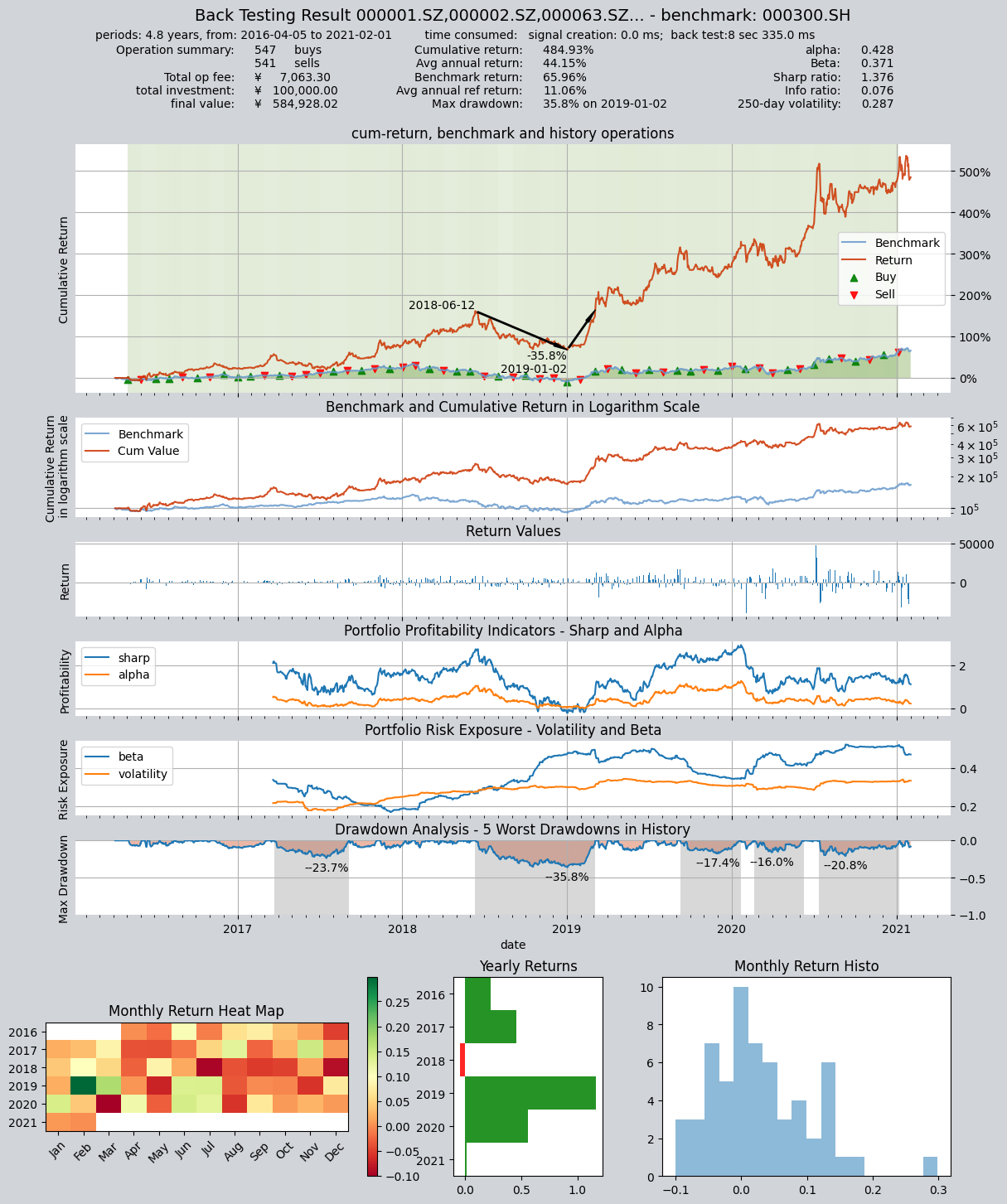
Configure otro período de prueba retrospectiva desde el 5 de abril de 2016 hasta el 1 de febrero de 2021 y ejecute la estrategia. Puedes ver que la estrategia es efectiva en diferentes períodos.
shares = qt.filter_stock_codes(index='000300.SH', date='20190501')
alpha = MultiFactors()  # 实例化策略
op = qt.Operator(alpha, signal_type='PT')  # 创建Operator交易员对象,使用PT信号类型(仓位目标信号)
op.op_type = 'stepwise'
op.set_blender('1.0*s0')  # 设置仓位调整公式,仓位目标为1.0*s0,即持仓百分比总和等于100%
op.run(mode=1,
       invest_start='20160405',  # 回测起始时间
       invest_end='20210201',  # 回测结束时间
       asset_type='E',  # 股票
       asset_pool=shares,  # 股票池
       trade_batch_size=100,  # 交易最小批量
       sell_batch_size=1,  # 卖出最小批量
       trade_log=True,  # 产生交易记录
      )

print()
Los resultados son los siguientes:
         ====================================
         |                                  |
         |       BACK TESTING RESULT        |
         |                                  |
         ====================================

    qteasy running mode: 1 - History back testing
    time consumption for operate signal creation: 0.0 ms
    time consumption for operation back looping:  8 sec 335.0 ms

    investment starts on      2016-04-05 00:00:00
    ends on                   2021-02-01 00:00:00
    Total looped periods:     4.8 years.

    -------------operation summary:------------
    Only non-empty shares are displayed, call
    "loop_result["oper_count"]" for complete operation summary

              Sell Cnt Buy Cnt Total Long pct Short pct Empty pct
    000063.SZ    2        2      4     3.4%      0.0%     96.6%
    000100.SZ    3        3      6     5.2%      0.0%     94.8%
    000157.SZ    1        1      2     1.8%      0.0%     98.2%
    000333.SZ    2        2      4     3.4%      0.0%     96.6%
    000338.SZ    1        1      2     1.7%      0.0%     98.3%
    000413.SZ    2        2      4     3.6%      0.0%     96.4%
    000596.SZ    1        1      2     1.8%      0.0%     98.2%
    000625.SZ    3        3      6     5.3%      0.0%     94.7%
    000629.SZ    1        1      2     1.7%      0.0%     98.3%
    000651.SZ    1        1      2     1.7%      0.0%     98.3%
    ...            ...     ...   ...      ...       ...       ...
    688005.SH    1        2      3     3.3%      0.0%     96.7%
    000733.SZ    1        1      2     1.8%      0.0%     98.2%
    002180.SZ    1        1      2     1.7%      0.0%     98.3%
    600039.SH    1        1      2     1.7%      0.0%     98.3%
    600803.SH    1        1      2     1.7%      0.0%     98.3%
    601615.SH    1        1      2     1.8%      0.0%     98.2%
    000983.SZ    2        2      4     3.3%      0.0%     96.7%
    600732.SH    3        4      7     6.7%      0.0%     93.3%
    600754.SH    1        1      2     1.8%      0.0%     98.2%
    601699.SH    1        1      2     1.7%      0.0%     98.3%

    Total operation fee:     ¥    7,063.30
    total investment amount: ¥  100,000.00
    final value:              ¥  584,928.02
    Total return:                   484.93%
    Avg Yearly return:               44.15%
    Skewness:                         -0.14
    Kurtosis:                          2.77
    Benchmark return:                65.96%
    Benchmark Yearly return:         11.06%

    ------strategy loop_results indicators------
    alpha:                            0.428
    Beta:                             0.371
    Sharp ratio:                      1.376
    Info ratio:                       0.076
    250 day volatility:               0.287
    Max drawdown:                    35.84%
        peak / valley:        2018-06-12 / 2019-01-02
        recovered on:         2019-03-05

    ===========END OF REPORT=============